Part 2 - Python tools for data science

DAT565_2

Introduction

In this part we’re going to explore some popular Python tools for data science.

NumPy

Numerical Python, is the standard package for computation and array operations.

Low-level functions are written in C, therefore, very fast.

Basic operations in NumPy

We usually import as:

1
import numpy as np

NumPy arrays can be constructed with the following:

1
A = np.array([69, 420, 1337, 42])

A NumPy array is defined by:

The number of dimensions it has (ndim)
The number of elements it has (size)
Its shape (number of elements along an axis)
Its dtype

1
A = np.array([69, 420, 1337, 42])
2
# A.ndim = 1
3
# A.size = 4
4
# A.shape = (4, )
5
# A.dtype = int64

We can either specify the dtype or let NumPy automatically assign it.

Different ways to create NumPy arrays that we usually use:

arange construct numbers from a range.
zeros creates an array full of zeros, with any shape.
ones creates an array full of ones, with any shape.
eye creates the identity array.
full creates an array filled with a specific element/array.

We can reshape our arrays and matrix, the new shape must have equal size (product of the shape).

1
A = np.array([69, 420, 1337, 42])
2
A.reshape(2, 2)
3
'''
4
[[69, 420],
5
 [1337, 42]]
6
'''

This does not make a copy, this returns a view (basically a pointer).

We can transpose our arrays and matrix as well:

1
A = np.array([69, 420, 1337, 42])
2
A.reshape(2, 2).T
3
'''
4
[[69, 1337],
5
 [420, 42]]
6
'''

We can change the dtype with the .astype() function:

1
A = np.array([69, 420, 1337, 42])
2
A.astype(np.float32)
3
'''
4
[69.0, 420.0, 1337.0, 42.0]
5
'''

We access elements in NumPy arrays with usual bracket notation:

1
A = np.array([69, 420, 1337, 42])
2
A[0]
3
'''
4
69
5
'''

NumPy supports Python style slicing:

1
A = np.array([69, 420, 1337, 42])
2
# A[1:-1] = [420, 1337]
3
# A[::2] = [69, 1337]

NumPy supports all basic math operations:

1
A = np.array([69, 420, 1337, 42])
2
# A + 1 = [70, 421, 1338, 43]

There are a lot more functions to explore :)

Matplotlib

Matplotlib is the standard way of plotting figures and graphs in Python. Used for ploting any kind of plot you can think of, scatter plots, line plots, contour plots, etc.

It comes with multiple APIs, but the standard one for Python is the pyplot API. Let’s take a look at a practical example.

Anscombe’s quartet

Anscombe’s quartet is a small dataset that shows the importance of graphing your data when dealing with statistics.

To understand we’ll graph this dataset for ourselves:

1
import numpy as np
2
import matplotlib.pyplot as plt

Firstly, let’s import numpy for the data processing and matplot for the plotting.

1
anscombe_data = np.array([10.0, 8.04, 10.0, 9.14, 10.0, 7.46, 8.0, 6.58,
2
8.0, 6.95, 8.0, 8.14, 8.0, 6.77, 8.0, 5.76,
3
13.0, 7.58, 13.0, 8.74, 13.0, 12.74, 8.0, 7.71,
4
9.0, 8.81, 9.0, 8.77, 9.0, 7.11, 8.0, 8.84,
5
11.0, 8.33, 11.0, 9.26, 11.0, 7.81, 8.0, 8.47,
6
14.0, 9.96, 14.0, 8.10, 14.0, 8.84, 8.0, 7.04,
7
6.0, 7.24, 6.0, 6.13, 6.0, 6.08, 8.0, 5.25,
8
4.0, 4.26, 4.0, 3.10, 4.0, 5.39, 19.0, 12.50,
9
12.0, 10.84, 12.0, 9.13, 12.0, 8.15, 8.0, 5.56,
10
7.0, 4.82, 7.0, 7.26, 7.0, 6.42, 8.0, 7.91,
11
5.0, 5.68, 5.0, 4.74, 5.0, 5.73, 8.0, 6.89])

Let’s reshape our NumPy array so it is a bit more readble and how it looks in Wikipedia.

1
anscombe_data = anscombe_data.reshape(11, 4, 2).transpose(1, 0, 2)
2
'''
3
[[[10.    8.04]
4
  [ 8.    6.95]
5
  [13.    7.58]
6
  [ 9.    8.81]
7
  [11.    8.33]
8
  [14.    9.96]
9
  [ 6.    7.24]
10
  [ 4.    4.26]
11
  [12.   10.84]
12
  [ 7.    4.82]
13
  [ 5.    5.68]]
14

15
 [[10.    9.14]
16
  [ 8.    8.14]
17
  [13.    8.74]
18
  [ 9.    8.77]
19
  [11.    9.26]
20
  [14.    8.1 ]
21
  [ 6.    6.13]
22
  [ 4.    3.1 ]
23
  [12.    9.13]
24
  [ 7.    7.26]
25
  [ 5.    4.74]]
26

27
 [[10.    7.46]
28
  [ 8.    6.77]
29
  [13.   12.74]
30
  [ 9.    7.11]
31
  [11.    7.81]
32
  [14.    8.84]
33
  [ 6.    6.08]
34
  [ 4.    5.39]
35
  [12.    8.15]
36
  [ 7.    6.42]
37
  [ 5.    5.73]]
38

39
 [[ 8.    6.58]
40
  [ 8.    5.76]
41
  [ 8.    7.71]
42
  [ 8.    8.84]
43
  [ 8.    8.47]
44
  [ 8.    7.04]
45
  [ 8.    5.25]
46
  [19.   12.5 ]
47
  [ 8.    5.56]
48
  [ 8.    7.91]
49
  [ 8.    6.89]]]
50
'''

Let’s break it up into the four indviual datasets:

1
anscombe = {'I': anscombe_data[0, :, :],
2
            'II': anscombe_data[1, :, :],
3
            'III': anscombe_data[2, :, :],
4
            'IV': anscombe_data[3, :, :]}

Before we plot the actual graphs, let’s take a loook at the mean, standard devation and variance for all four of the datasets.

1
for key, value in anscombe.items():
2
    print(key)
3
    print('Mean: ', np.mean(value, axis=0))
4
    print('Standard deviation: ', np.std(value, ddof=1, axis=0))
5
    print('Variance: ', np.var(value, axis=0))
6
    print('Correlation coefficient: ', np.corrcoef(
7
        value[:, 0], value[:, 1])[0, 1])
8
    print()
9
'''
10
I
11
Mean:  [9.         7.50090909]
12
Standard deviation:  [3.31662479 2.03156814]
13
Variance:  [10.          3.75206281]
14
Correlation coefficient:  0.81642051634484
15

16
II
17
Mean:  [9.         7.50090909]
18
Standard deviation:  [3.31662479 2.03165674]
19
Variance:  [10.          3.75239008]
20
Correlation coefficient:  0.8162365060002428
21

22
III
23
Mean:  [9.  7.5]
24
Standard deviation:  [3.31662479 2.0304236 ]
25
Variance:  [10.          3.74783636]
26
Correlation coefficient:  0.8162867394895984
27

28
IV
29
Mean:  [9.         7.50090909]
30
Standard deviation:  [3.31662479 2.03057851]
31
Variance:  [10.          3.74840826]
32
Correlation coefficient:  0.8165214368885028
33
'''

So, from a purerly statistical view, we would think that all these datasets should look somewhat similar, right?

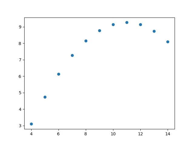
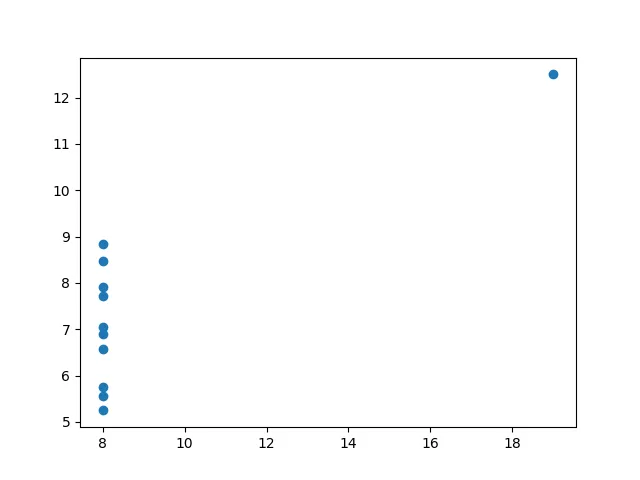
Let’s plot them and see. Let’s plot them as scatter plots:

1
for key, value in anscombe.items():
2
    plt.scatter(value[:, 0], value[:, 1])
3
    plt.sho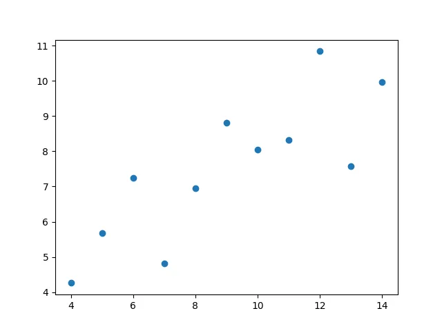w()

Let’s plot them all together:

1
fig, axs = plt.subplots(2, 2)
2
for (ax, (key, value)) in zip(axs.ravel(), anscombe.items()):
3
    ax.scatter(value[:, 0], value[:, 1])
4
    ax.set_xlabel('$x$')
5
    ax.set_ylabel('$y$')
6
    ax.set_title(key)
7

8
fig.tight_layout()
9
plt.sho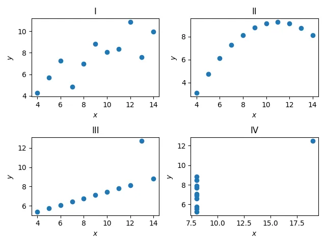w()

So, we can see that these datasets, in reality, differ a lot from each other, but seem to have equivalent statistical properties. We’ll look into more statistics later on :).

Pandas

The last library we’ll cover is the data analysis library Pandas. When dealing with large datasets, we’ll usually want to use common convient functions to read, write and manipulate data fast.

Pandas can make use of NumPy as a backend for some data.

Before jumping into a practial example we’re we’ll use Pandas, let’s first understand how we’ll represent data.

Wide and long format

When we want to represent data, we have two options:

In wide format, the data is indexed by first column where the values do not repeat.
- Different variables for observations are placed on different columns.
In long format, a column indexes the different kinds of observations and another column contains the respective values.

Converting data to wide format is called pivoting.

Converting data to long format is unpivoting or melting.

1
'''
2
Wide format
3

4
  Person  Age  Weight  Height
5
0    Bob   32     168     180
6
1  Alice   24     150     175
7
2  Steve   64     144     165
8

9
Long format
10

11
  Person Attribute  Value
12
0    Bob       Age     32
13
1    Bob    Weight    168
14
2  Alice       Age     24
15
3  Alice    Weight    150
16
4  Steve       Age     64
17
5  Steve    Weight    144
18
'''

Palmer penguins

We’ll use the palmer penguins data set.

Let’s import Pandas, note that we don’t import NumPy here!

1
import pandas as pd

Pandas offers a great selection of reading methods for different file formats.

1
df = pd.read_csv('penguins_size.csv')
2
print(df)
3
'''
4
    species     island  culmen_length_mm  culmen_depth_mm  flipper_length_mm  body_mass_g     sex
5
0    Adelie  Torgersen              39.1             18.7              181.0       3750.0    MALE
6
1    Adelie  Torgersen              39.5             17.4              186.0       3800.0  FEMALE
7
2    Adelie  Torgersen              40.3             18.0              195.0       3250.0  FEMALE
8
3    Adelie  Torgersen               NaN              NaN                NaN          NaN     NaN
9
4    Adelie  Torgersen              36.7             19.3              193.0       3450.0  FEMALE
10
..      ...        ...               ...              ...                ...          ...     ...
11
339  Gentoo     Biscoe               NaN              NaN                NaN          NaN     NaN
12
340  Gentoo     Biscoe              46.8             14.3              215.0       4850.0  FEMALE
13
341  Gentoo     Biscoe              50.4             15.7              222.0       5750.0    MALE
14
342  Gentoo     Biscoe              45.2             14.8              212.0       5200.0  FEMALE
15
343  Gentoo     Biscoe              49.9             16.1              213.0       5400.0    MALE
16
'''

To get an overview we can use the .describe() function.

1
print(df.describe())
2
'''
3
       culmen_length_mm  culmen_depth_mm  flipper_length_mm  body_mass_g
4
count        342.000000       342.000000         342.000000   342.000000
5
mean          43.921930        17.151170         200.915205  4201.754386
6
std            5.459584         1.974793          14.061714   801.954536
7
min           32.100000        13.100000         172.000000  2700.000000
8
25%           39.225000        15.600000         190.000000  3550.000000
9
50%           44.450000        17.300000         197.000000  4050.000000
10
75%           48.500000        18.700000         213.000000  4750.000000
11
max           59.600000        21.500000         231.000000  6300.00000
12
'''

To select a column we can do:

1
print(df['species'])
2
'''
3
0      Adelie
4
1      Adelie
5
2      Adelie
6
3      Adelie
7
4      Adelie
8
        ...
9
339    Gentoo
10
340    Gentoo
11
341    Gentoo
12
342    Gentoo
13
343    Gentoo
14
Name: species, Length: 344, dtype: object
15
'''

We can also select data with .iloc and .loc. iloc is index based.

1
print(df.iloc[0])
2
'''
3
species                 Adelie
4
island               Torgersen
5
culmen_length_mm          39.1
6
culmen_depth_mm           18.7
7
flipper_length_mm        181.0
8
body_mass_g             3750.0
9
sex                       MALE
10
Name: 0, dtype: object
11
'''

Where as .loc is string based, in this case both iloc and loc yields the same answer since we group the data with index. In other datasets we could have a string based index.

We can easily filter and choose the right data with:

1
print(df.loc[df['culmen_length_mm'] < 40])
2
'''
3
    species     island  culmen_length_mm  culmen_depth_mm  flipper_length_mm  body_mass_g     sex
4
0    Adelie  Torgersen              39.1             18.7              181.0       3750.0    MALE
5
1    Adelie  Torgersen              39.5             17.4              186.0       3800.0  FEMALE
6
4    Adelie  Torgersen              36.7             19.3              193.0       3450.0  FEMALE
7
5    Adelie  Torgersen              39.3             20.6              190.0       3650.0    MALE
8
6    Adelie  Torgersen              38.9             17.8              181.0       3625.0  FEMALE
9
..      ...        ...               ...              ...                ...          ...     ...
10
146  Adelie      Dream              39.2             18.6              190.0       4250.0    MALE
11
147  Adelie      Dream              36.6             18.4              184.0       3475.0  FEMALE
12
148  Adelie      Dream              36.0             17.8              195.0       3450.0  FEMALE
13
149  Adelie      Dream              37.8             18.1              193.0       3750.0    MALE
14
150  Adelie      Dream              36.0             17.1              187.0       3700.0  FEMALE
15

16
[100 rows x 7 columns]
17
'''

We can have chained boolean expressions with & for AND, | for OR, and ~ for NOT.

1
print(df.loc[(df['culmen_length_mm'] < 60) & (df['species'] == 'Gentoo')])
2
'''
3
    species  island  culmen_length_mm  culmen_depth_mm  flipper_length_mm  body_mass_g     sex
4
220  Gentoo  Biscoe              46.1             13.2              211.0       4500.0  FEMALE
5
221  Gentoo  Biscoe              50.0             16.3              230.0       5700.0    MALE
6
222  Gentoo  Biscoe              48.7             14.1              210.0       4450.0  FEMALE
7
223  Gentoo  Biscoe              50.0             15.2              218.0       5700.0    MALE
8
224  Gentoo  Biscoe              47.6             14.5              215.0       5400.0    MALE
9
..      ...     ...               ...              ...                ...          ...     ...
10
338  Gentoo  Biscoe              47.2             13.7              214.0       4925.0  FEMALE
11
340  Gentoo  Biscoe              46.8             14.3              215.0       4850.0  FEMALE
12
341  Gentoo  Biscoe              50.4             15.7              222.0       5750.0    MALE
13
342  Gentoo  Biscoe              45.2             14.8              212.0       5200.0  FEMALE
14
343  Gentoo  Biscoe              49.9             16.1              213.0       5400.0    MALE
15

16
[123 rows x 7 columns]
17
'''

Very often it is useful to sort/index the raw data based on some metric, let’s group the numerical data by the species and take the mean:

1
print(df.groupby('species')[['culmen_length_mm', 'culmen_depth_mm', 'flipper_length_mm', 'body_mass_g']].mean())
2
'''
3
           culmen_length_mm  culmen_depth_mm  flipper_length_mm  body_mass_g
4
species
5
Adelie            38.791391        18.346358         189.953642  3700.662252
6
Chinstrap         48.833824        18.420588         195.823529  3733.088235
7
Gentoo            47.504878        14.982114         217.186992  5076.016260
8
'''

Let’s format this into long format:

1
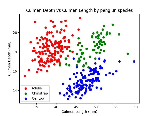
df2 = df.groupby('species')[['culmen_length_mm', 'culmen_depth_mm', 'flipper_length_mm', 'body_mass_g']].mean()
2
print(df2.reset_index().melt(id_vars=['species'], var_name='measurement', value_name='value'))
3
'''
4
      species        measurement        value
5
0      Adelie   culmen_length_mm    38.791391
6
1   Chinstrap   culmen_length_mm    48.833824
7
2      Gentoo   culmen_length_mm    47.504878
8
3      Adelie    culmen_depth_mm    18.346358
9
4   Chinstrap    culmen_depth_mm    18.420588
10
5      Gentoo    culmen_depth_mm    14.982114
11
6      Adelie  flipper_length_mm   189.953642
12
7   Chinstrap  flipper_length_mm   195.823529
13
8      Gentoo  flipper_length_mm   217.186992
14
9      Adelie        body_mass_g  3700.662252
15
10  Chinstrap        body_mass_g  3733.088235
16
11     Gentoo        body_mass_g  5076.016260
17
'''

Lastly, let’s make a simple plot that shows the culmen depth vs culmen length for all the species in one scatter plot.

1
import matplotlib.pyplot as plt
2
import numpy as np
3
colors = ['red', 'green', 'blue']
4
species_to_num = {v: k for (k, v) in enumerate(df['species'].unique())}
5

6
for species, group in df.groupby('species'):
7
    plt.scatter(group['culmen_length_mm'], group['culmen_depth_mm'],
8
                color=colors[species_to_num[species]], label=species)
9
    plt.xlabel('Culmen Length (mm)')
10
    plt.ylabel('Culmen Depth (mm)')
11
    plt.title('Culmen Depth vs Culmen Length by pengiun species')
12
    plt.legend()
13

14
plt.show()