Introduction
Games are a very human thing to play (and design). So it is a very natural thing to approach them as systems that can be designed and analyzed.
One of the earliest examples is the mechanical Turk, a chess-playing machine that was actually a hoax 1.
Then in the 1900s, we had the first computer programs that could play chess. Most famously, IBM’s Deep Blue that beat the world champion Garry Kasparov in 1997 2.

A more modern game-playing system is OpenAI Five, a team of five AI agents that can play the game Dota 2 3.
Formalizing Games
But to approach games as systems, we first need to formalize them. One of the most common games (and easiest to formalize) are zero-sum games.
A zero-sum game is a mathematical representation of a situation in which each participant’s gain or loss of utility is exactly balanced by the losses or gains of the utility of the other participants.
Or, in other (simpler) words, one player winning implies one player losing.
Games are inherently about actions, our goal is to select actions that improve our chances of winning.
To win, we need to account for good and bad features when selecting actions.
Think of Tic-Tac-Toe, to play optimally, we must pick the best path, but which is it?

We need to (formalize) and introduce search trees.
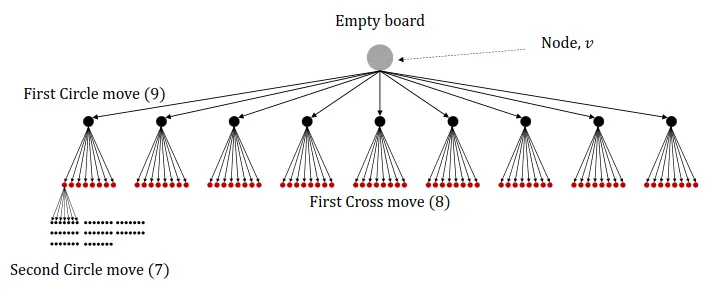
At some point in the tree, an end state is reached, we call these terminal nodes.
The value of a terminal node is the utility of the game, i.e., if it leads to a win, loss, or draw.
A search tree can be used to enumerate possible futures. By identifying good futures (wins), we can backtrack, which actions do we have to take to reach that future?
However, a plan is only a plan, we can’t control the opponent’s actions, thus, the answer is also dependent on the opponent’s actions.
Let’s, for now, assume that our opponent has a fixed, known policy $\pi$.
Thus, for each position,
- Compute the probability of reaching winning states.
- Based on the probability of the future states.
- Execute the action(s) with the highest success rate.
But, if our opponent is adaptive, i.e., used to be suboptimal but changes to being optimal, our probabilities will change.
Minimax optimization
To guarantee success against the best possible opponent, we formulate the following strategy,
Minimize the maximum success of your opponent (worst-case scenario).
Assume that we knew the best possible move and that our opponent will play that move. Then we proceed as before, count future success rate of each action and act accordingly.
But what is the best move?
Let’s formalize it, four our purposes, a decision process describes an agent taking actions $A_t$, according to a policy $\pi$ in states $S_t$, observed through $X_t$. Which transitions according to the dynamics $p(S_t | S_{<t}, A_{<t})$.
We will often have a designated reward $R_t$, a function of $X_t$ that we want to optimize.
In two-player games, there are two agents with (potentially) different policies, $\pi$ (player) and $\mu$ (opponent).
$\bar{R}(\pi, \mu)$ denotes the average reward (e.g., win rate) of $\pi$ against $\mu$.
Minimax play for $\pi$ against $\mu$ optimizes,
$$ \underset{\pi}{\min} \ \underbrace{{\underset{\mu}{\max} \ \bar{R}(\pi, \mu)}}_{\text{Strongest Opponent}}. $$
Minimax Planning
In search trees, minimax planning select the next action at time $t$ by examining the best path $A_t, \ldots, A_T$ for the player and the best path $B_{t + 1}, \ldots, B_T$ for the opponent until end $T$,
$$ \underset{A_t, \ldots, A_T}{\min} \ \underset{B_{t + 1}, \ldots, B_T}{\max} \ \bar{R}(A, B). $$
However, this is computationally infeasible for most games, as the search tree grows exponentially with the number of actions. For Tic-Tac-Toe the total number of possible states (boards) < 20000, but for chess, it is $\approx 10^{120}$.
One strategy is to truncate at finite depth, that means, we limit ourselves to only looking $d$ steps ahead. The drawback of this approach is, how do we value non-terminal nodes?
For humans, it is easy to see that some moves are better than others, but how do we quantify this? In early systems, we actually used human knowledge to assign values to non-terminal nodes.
Learning to Play
As mentioned, the two problems with large state space are,
- It is infeasible to explore every state.
- We can’t look at every possible future (in a feasible time span).
- It is infeasible to store the value of each state.
- We can’t store the value of every possible future (in a feasible memory space).
Let’s tackle each problem.
Exploration
One way to tackle the exploration problem is to sample the state space, i.e., we only try a subset of actions. But how do we make sure we don’t leave out good ones?
Monte Carlo Tree Search
Monte-Carlo methods deal with random sampling.
Instead of searching exhaustively, our search based on experiments with randomly selected actions.
Essentially, we try playing something and remember what happened.
The MCTS algorithm is based on four steps,
- Selection
- Finding unexplored nodes (state-action pairs that haven’t been tried).
- Based on what we know so far, traverse down until an unexplored child node is reached.
- We use a tree policy for selection.
- Expansion
- Once we have selected node, we expand it.
- We add a new child node to the tree.
- Now we need to evaluate this new node.
- Simulation/Rollout
- We simulate the game from the new node.
- Based on our simulation policy (usually a simple random policy), we continue playing until we hit a terminal node.
- At the terminal node, we know the value!
- Backpropagation
- We update the value of the nodes we traversed.
- We backpropagate the value of the terminal node to the root node.
- Statistics of our nodes are updated, $N(v)$ - number of times visited, $Q(v)$ - total reward starting from $v$, also called Q-value.
Tree Policies
Just selecting nodes randomly is very inefficient, the statistics we collect can be used to improve our selection during MCTS (and thus the action we choose to play in the end).
How can we balance trying new things (exploration) and using our prior knowledge (exploitation)?
Greedy policies
A greedy policy selects the best action according to some metric.
For example, the highest average reward accumulated so far,
$$ A = \underset{a}{\arg \max} \ \frac{Q(v_a)}{N(v_a)}. $$
However, this leads to no exploration, but this is good when $Q$ is a very good approximation of the value.
$\epsilon$-greedy policies
A $\epsilon$-greedy policy chooses the greedy action with probability $1 - \epsilon$ and a random action with probability $\epsilon$.
Trades off exploration and exploitation (a bit).
However, there’s a problem, we may try an action known to be bad, by chance.
Upper Confidence Bounds (UCB)
The UCB is a popular heuristic, bound on the true $Q$-value for an action $a$ in node $v$,
$$ Q(v_a) \leq \hat{Q}_t(v_a) + \hat{U}_t(v_a), $$
where $Q(v_a)$ is the true value, $\hat{Q}_t(v_a)$ is the estimated value, and $\hat{U}_t(v_a)$ is the uncertainty.
We act greedily,
$$ a_t = \underset{a}{\arg \max} [\hat{Q}_t(v_a) + \hat{U}_t(v_a)]. $$
We can define $\hat{U}_t(v_a)$ as,
$$ \hat{U}_t(v_a) = c \sqrt{\frac{\log N(v)}{N(v_a)}}, $$
where $c$ is a hyperparameter that controls the balance between exploration and exploitation. If you are wondering where this comes from, it is derived from the Hoeffding inequality 4.
The application of UCB to search trees is called UCT (Upper Confidence Trees). One variant is defined as (but there are many),
$$ \text{UCT}(v_i, v) = \frac{Q(v_i)}{N(v_i)} + c \sqrt{\frac{\log N(v)}{N(v_i)}}. $$
MCTS is repeat until sufficient statistics have been gathered, each potential action $a$ has statistics $N(v_a)$ and $Q(v_a)$.
We now can choose the action corresponding to the most visited state.
Function Approximation
Remember the second problem with large state spaces, we can’t store the value of every possible future.
The problem of many/high-dimensional states is common in AI problems, e.g., image classification, speech recognition, etc.
Intuitively, the details of each state matter less, the more information there is. A lot of states are similar to each other.
As humans, we recognize these similarities, and disregard irrelevant information.
A very natural thing from machine learning is function approximation, we can learn a function that approximates the $Q$-value.
During backpropagation, we don’t just update counters $N,Q$, but also the parameters of neural nets predicting the $Q$-value.
Since we now don’t need any human intervention or knowledge, self-play is possible.
Markov Property
One last thing to mention is the Markov property.
In Chess, Go, Tic-Tac-Toe, the history of a game does not influence transitions, states are Markovian,
$$ p(S_t | S_1, \ldots, S_{t-1}, A_1, \ldots, A_{t-1}) = p(S_t | S_{t-1}, A_{t-1}). $$
For example, if you move a chess piece from E2 to E4, nothing else happens. The set of valid moves can be read of the board beforehand.
Non-Markov (Long) Games
When Markovianity doesn’t hold, long games becomes hard.
We have to memorize/summarize history to predict the future. Although, this is starting to be addressed more by modern systems.
Conclusion
Use machine learning where it helps!
It is a great tool at condensing information and extracting relevant patterns.
AlphaGO combined traditional MCTS with ML, and it beat the world champion 5.