Part 7 - Bode plot | rezarezvan.com

Introduction

In this part we’ll begin with the part about frequency analysis.

Test functions

Often when we want to test our system to determine the overall stability, time it takes and the response we get.

We often test with our unit step function:

\sigma(t) = \begin{cases} 1 & t \geq 0 \newline 0 & t < 0. \end{cases}

We call a system response to the unit step function for unit step response.

Given a system of form:

G(s) = \dfrac{K}{1 + Ts}.

We get a unit step response of $y(t) = K(1 - e^{-t/T})$ .

We also have our beloved impulse function, $\delta(t)$ .

\delta(t) = \lim_{\epsilon \to 0} \begin{cases} \dfrac{1}{\epsilon} & 0 \leq t \leq \epsilon \newline 0 & t > \epsilon, t < 0. \end{cases}

We also have the properties:

\begin{align*} \int_{-\infty}^{\infty} \delta(t) \, dt & = 1, \newline \int_{-\infty}^{\infty} \delta(t - T) f(t) \, dt & = f(T), \newline \mathcal{L}\{\delta(t)\} = \int_0^{\infty} \delta(t) e^{-st} \, dt & = e^{-s \cdot 0} = 1. \end{align*}

Delay rate

We can “delay” a function using a unit step with a delay:

\mathcal{L}\{y(t - T)\sigma(t - T)\} = e^{-Ts} \cdot \mathcal{L}\{y(t)\} = e^{-Ts} Y(s).

Definition 1 (Stable system)

A system is stable if:

\lim_{t \to \infty} \{\text{Impulse response}\} = 0.

Ramp function

Another function that we’ll perform a lot of tests with is the ramp function. Which we define as:

t \sigma(t).

The Laplace transform of this is (using partial integration):

\mathcal{L} \{t \sigma(t) \} = \dfrac{1}{s^2}.

Example 1

Determine the long term error, when the insignal is a ramp function, $t \sigma(t)$ .

Given that:

F(s) = \dfrac{s + 2}{s}, \quad G(s) = \dfrac{1}{s + 1}.

We know that:

\begin{align*} E(s) & = R(s) - Y(s), \newline Y(s) & = \dfrac{L(s)}{1 + L(s)} \cdot R(s), \newline L(s) & = F(s)G(s) = \dfrac{s + 2}{s(s + 1)}. \end{align*}

So:

\begin{align*} E(s) & = R(s) - \dfrac{L(s)}{1 + L(s)} \cdot R(s) \newline & = R(s) \left(1 - \dfrac{L(s)}{1 + L(s)} \right) \newline & = R(s) \left(\dfrac{1}{1 + L(s)} \right) \newline & = \dfrac{1}{s^2} \left(\frac{1}{1 + \frac{s + 2}{s(s + 1)}} \right) \newline & = \dfrac{1}{s^2} \left(\frac{s(s + 1)}{s(s + 1) + s + 2} \right) \newline & = \dfrac{1}{s^2} \left(\frac{s(s + 1)}{s^2 + 2s + 2} \right) \newline & = \frac{(s + 1)}{s(s^2 + 2s + 2)}. \end{align*}

Using the final value theorem:

\begin{align*} e(\infty) = \lim_{t \to \infty} e(t) & = \lim_{s \to 0} s \cdot E(s) \newline & = \lim_{s \to 0} s \cdot \frac{(s + 1)}{s(s^2 + 2s + 2)} \newline & = \lim_{s \to 0} \frac{(s + 1)}{(s^2 + 2s + 2)} \newline & = \boxed{\dfrac{1}{2}}. \end{align*}

Frequency analysis

Definition 2 (Frequency function)

The frequency function, $G(j\omega)$ for a system is given by:

G(j\omega) = G(s) \biggr\rvert_{s = j \omega}.

The polar form of this function will be written as:

G(j\omega) = |G(j\omega)| \cdot e^{j \arg(G(j\omega))}.

Example 2

Let $u(t) = A \sin(\omega t + \phi)$ with the system, $G(s)$ what will our $y(t)$ be?

y(t) = |G(j\omega)| \cdot A \sin(\omega t + \phi + \arg(G(j\omega))) (+ e^{-\lambda t}).

That last part is called the transient part and should in reality just be zero.

Bode plot

Bode plots are plots that show the system magnitude and phase shift in a system.

Usually the magnitude can/will be in decibels.

Example 3

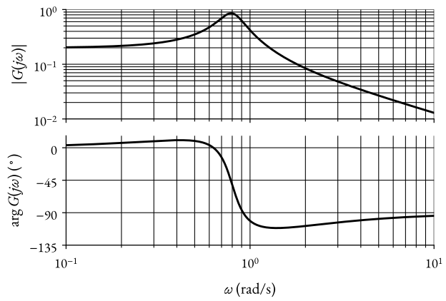Figure 1: An example Bode plot: magnitude (top) and phase (bottom).

Where the $y$ -axis is either the phase ( $\arg(G(j\omega))$ ) or the magnitude ( $|G(j \omega)|$ ).

Remember that decibels are just:

\mathrm{dB} = 20 \log_{10}(|G(j\omega)|).

Example 4

Given:

G(s) = \dfrac{1}{s(s + 2)}.

This means that:

G(j\omega) = \dfrac{1}{j\omega(j\omega + 2)}.

The magnitude is:

|G(j\omega)| = \dfrac{1}{\omega \sqrt{\omega^2 + 2^2}} = \dfrac{1}{\omega \sqrt{4 + \omega^2}}.

The phase is:

\begin{align*} \arg(G(j\omega)) & = \arg\left( \dfrac{1}{j\omega(j\omega + 2)} \right) \newline & = \arg(1) - \arg(j\omega(j\omega + 2)) \newline & = \arg(1) - (\arg(j\omega) + \arg(j\omega + 2)) \newline & = 0^\circ - \left(90^\circ + \arctan{\left(\dfrac{\omega}{2}\right)}\right) \newline & = -90^\circ - \arctan{\left(\dfrac{\omega}{2}\right)}. \end{align*}

If we now plot these:

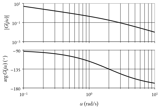Bode plot of G(s) = \frac{1}{s(s + 2)}. — Figure 2: Bode plot of $G(s) = \frac{1}{s(s + 2)}$ .

Type of factors

In our systems we’ll deal/want these type of factors:

s, \quad 1 + \dfrac{s}{\omega_1}, \quad e^{-Ts}, \quad s^2 + 2 \zeta \omega_n s + \omega_n^2.

Also, good to remember, if $\zeta > 1$ , then we can split up this second-order term into first-order term(s).

Let’s do the bode plot for each term.

G(s) = s, \quad G(j\omega) = j\omega, \quad |G(j\omega)| = \omega, \quad \arg(G(j\omega)) = 90^\circ.

Plotting this:

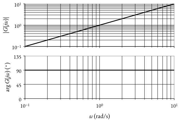Bode plot of G(s) = s. — Figure 3: Bode plot of $G(s) = s$ .

Simple!

Now, for $\dfrac{1}{s}$

G(s) = \dfrac{1}{s}, \quad G(j\omega) = \dfrac{1}{j\omega}, \quad |G(j\omega)| = \dfrac{1}{\omega}, \quad \arg(G(j\omega)) = -90^\circ.

Plotting this:

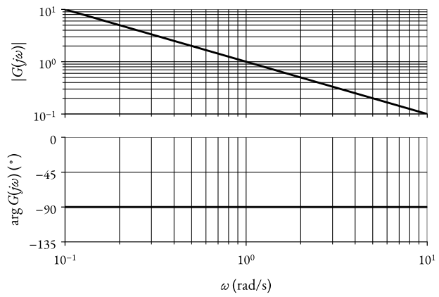Bode plot of G(s) = \frac{1}{s}. — Figure 4: Bode plot of $G(s) = \frac{1}{s}$ .

Now for $1 + \dfrac{s}{\omega_1}$

G(s) = 1 + \dfrac{s}{\omega_1}, \quad G(j\omega) = 1 + \dfrac{j\omega}{\omega_1}.

For this we’ll need to understand some cases.

Case $\omega \ll \omega_1$ :

G(j\omega) \approx 1, \quad |G(j\omega)| = 1, \quad \arg(G(j\omega)) = 0^\circ.

Case $\omega = \omega_1$ :

G(j\omega) = 1 + j, \quad |G(j\omega)| = \sqrt{1^2 + 1^2} = \sqrt{2}, \quad \arg(G(j\omega)) = 45^\circ.

Case $\omega \gg \omega_1$ :

G(j\omega) \approx j \dfrac{\omega}{\omega_1}, \quad |G(j\omega)| = \dfrac{\omega}{\omega_1}, \quad \arg(G(j\omega)) = 90^\circ.

Plotting for $\omega_1 = 2$ :

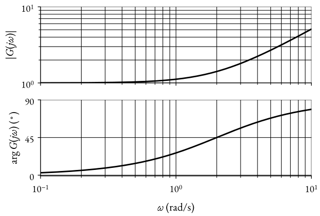Bode plot of G(s) = 1 + \frac{s}{\omega_1} for \omega_1 = 2. — Figure 5: Bode plot of $G(s) = 1 + \frac{s}{\omega_1}$ for $\omega_1 = 2$ .

This is what we’ll call for low and high frequency asymptotes.

Last factor before an example

G(s) = \dfrac{1}{1 + \dfrac{s}{\omega_1}}, \quad G(j\omega) = \dfrac{1}{1 + \dfrac{j\omega}{\omega_1}}.

Case $\omega \ll \omega_1$ :

G(j\omega) \approx 1, \quad |G(j\omega)| = 1, \quad \arg(G(j\omega)) = 0^\circ.

Case $\omega = \omega_1$ :

G(j\omega) = \dfrac{1}{1 + j}, \quad |G(j\omega)| = \dfrac{1}{\sqrt{1^2 + 1^2}} = \dfrac{1}{\sqrt{2}}, \quad \arg(G(j\omega)) = -45^\circ.

Case $\omega \gg \omega_1$ :

G(j\omega) \approx \dfrac{1}{j \dfrac{\omega}{\omega_1}}, \quad |G(j\omega)| = \dfrac{1}{\dfrac{\omega}{\omega_1}} = \dfrac{\omega_1}{\omega}, \quad \arg(G(j\omega)) = -90^\circ.

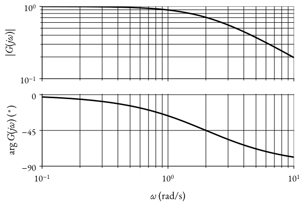Bode plot of G(s) = \frac{1}{1 + s / \omega_1} for \omega_1 = 2. — Figure 6: Bode plot of $G(s) = \frac{1}{1 + s / \omega_1}$ for $\omega_1 = 2$ .

Standard form

We’ll usually want to rewrite our transfer functions into these standard factor forms.

Let’s take an example to see why

Example 5

\begin{align*} G(s) & = \dfrac{3(1 + s)e^{-0.5s}}{s(s + 2)(s + 3)} \newline & = \dfrac{3(1 + s)e^{-0.5s}}{2s(1 + \frac{s}{2})(s + 3)} \newline & = \dfrac{3(1 + s)e^{-0.5s}}{6s(1 + \frac{s}{2})(1 + \frac{s}{3})} \newline & = \boxed{\dfrac{0.5(1 + s)e^{-0.5s}}{s(1 + \frac{s}{2})(1 + \frac{s}{3})}}. \end{align*}

This is now in standard form.

G(j\omega) = \boxed{\dfrac{0.5(1 + j\omega)e^{-0.5j\omega}}{j\omega(1 + \frac{j\omega}{2})(1 + \frac{j\omega}{3})}}.