Part 16 - Vector fields | rezarezvan.com

Introduction

In this part we’ll cover so-called vector fields.

Definition 1 (Vector field)

A vector field is a function, $F$ :

\begin{align*} F & : D \subset \mathbb{R}^2 \rarr \mathbb{R}^2 \quad \text{(2D)}, \newline F & : D \subset \mathbb{R}^3 \rarr \mathbb{R}^3 \quad \text{(3D)}. \end{align*}

Example 1

Consider $F(x, y) = (-y, x)$ (which is the same as $-y \vec{i} + x\vec{j}$ ).

The graph for this looks like:

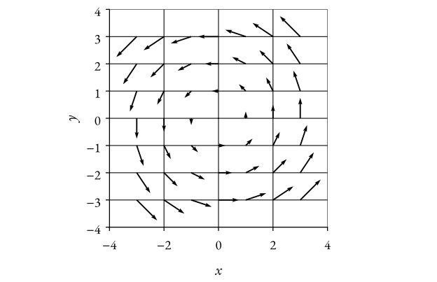The vector field \vec{F}(x, y) = \langle -y, x \rangle. — Figure 1: The vector field $\vec{F}(x, y) = \langle -y, x \rangle$ .

Gradient field

By this definition, we can say that.

Let $f: D \subset \mathbb{R}^2 \rarr \mathbb{R}$ be a differentiable function. The gradient is $\nabla f(x, y) = \langle f_x(x, y), f_y(x, y) \rangle$ .

The gradient is therefore a vector field!

\nabla f: D \rarr \mathbb{R}^2

Let’s quickly just do a simple gradient example to refresh our memory.

Example 2

Find $\nabla f$ for $f(x, y) = x^2 y - y^3$

\begin{align*} \nabla f(x, y) & = \langle f_x(x, y), f_y(x, y) \rangle \newline & = \langle 2xy, x^2 - 3y^2 \rangle. \end{align*}

Let’s also remember that $\nabla f(x, y)$ is perpendicular to the level curves of $f$ .

Which means, $\nabla f$ has larger (vector) length when the level curves are tighter together.

Definition 2 (Conservative vector field)

A vector field, $F$ , is called conservative, if there is a function, $f$ , for which $\nabla f = F$ .

In this case, $f$ , is called a potential for $F$ .

Integrating over vector fields

Suppose the vector field, $F$ , represents some force on the plane/space and suppose there is a string, curved of the shape of a curve, $C$ .

If a particle moves along the curve, the work done by $F$ , to move it a distance:

\int_C F \cdot dr

We call this the line integral of $F$ over $C$ .

Definition 3 (Line integral over a vector field)

If $C$ is parameterized as $\vec{r}(t) = \langle x(t), y(t), z(t) \rangle$ in the interval, $a \leq t \leq b$ . Then:

\int_C F \cdot dr = \int_a^b F(x(t), y(t), z(t)) \cdot \vec{r^\prime}(t) \, dt.

Example 3

Evaluate $\int_C F \cdot dr$ for $F(x, y, z) = (y, z, x)$ on the straight line from $(2, 0, 0)$ to $(3, 4, 5)$ .

Let’s first parameterize our curve.

\begin{align*} \vec{r}(t) & = \langle x_0 + ta, y_0 + tb, z_0 + tc \rangle \newline & = \langle 2 + t(3 - 2), 0 + t(4 - 0), 0 + t(5 - 0) \rangle \newline & = \langle 2 + t, 4t, 5t \rangle, \quad 0 \leq t \leq 1. \end{align*}

Which means:

\vec{r^\prime}(t) = \langle 1, 4, 5 \rangle, \quad 0 \leq t \leq 1.

Using our definition:

\begin{align*} \int_C F \cdot dr & = \int_0^1 \langle 4t, 5t, 2 + t \rangle \cdot \langle 1, 4, 5 \rangle \, dt \newline & = \int_0^1 4t + 20t + 10 + 5t \, dt \newline & = \int_0^1 29t + 10 \, dt \newline & = \dfrac{29}{2} t^2 + 10t \bigg\rvert_{t = 0}^{t = 1} \newline & = \boxed{\dfrac{29}{2} + 10} \end{align*}

Example 4

Evaluate $\int_C F \cdot dr$ for $F(x, y, z) = xy \vec{i} + yz \vec{j} + zx \vec{k}$ .

$C$ is given by, $\vec{r}(t) = \langle t, t^2, t^3 \rangle$ . For $0 \leq t \leq 1$ .

Let’s first rewrite $F$ :

F(x, y, z) = \langle xy, yz, zx \rangle

Let’s differentiate:

\vec{r^\prime}(t) = \langle 1, 2t, 3t^2 \rangle

Use our definition:

\begin{align*} \int_C F \cdot dr & = \int_0^1 \langle t^3, t^5, t^4 \rangle \cdot \langle 1, 2t, 3t^2 \rangle \, dt \newline & = \int_0^1 t^3 + 2t^6 + 3t^6 \, dt \newline & = \int_0^1 5t^6 + t^3 \, dt \newline & = \dfrac{5}{7} t^7 + \dfrac{1}{4} t^4 \bigg\rvert_{t = 0}^{t = 1} \newline & = \boxed{\dfrac{5}{7} + \dfrac{1}{4}} \end{align*}