Introduction
In this part we’ll cover Green’s Theorem, which will allow us to have a relationship between integrals and double integrals.
Before starting, we will only work with simple curves. Which essentially just means that the curves have no self-injections (only exception is when it starts and ends at the same point).
If C C C C C C D D D ∂ D = C \partial D = C ∂ D = C D D D
NB: “Positive” orientation is counter-clockwise and “Negative” orientation is clockwise.
Theorem 1 (Green’s Theorem) Let C C C D D D P , Q : D → R P, Q: D \rarr \mathbb{R} P , Q : D → R
∫ C P d x + Q d y = ∬ D ∂ Q ∂ x − ∂ P ∂ y d x d y . \int_C P \, dx + Q \, dy = \iint_D \dfrac{\partial Q}{\partial x} - \dfrac{\partial P}{\partial y} \, dx \, dy. ∫ C P d x + Q d y = ∬ D ∂ x ∂ Q − ∂ y ∂ P d x d y . Equivalently:
∫ ∂ D P d x + Q d y = ∬ D ∂ Q ∂ x − ∂ P ∂ y d x d y . \int_{\partial D} P \, dx + Q \, dy = \iint_D \dfrac{\partial Q}{\partial x} - \dfrac{\partial P}{\partial y} \, dx \, dy. ∫ ∂ D P d x + Q d y = ∬ D ∂ x ∂ Q − ∂ y ∂ P d x d y . Example 1 Evaluate ∫ C x 4 d x + x y d y \int_C x^4 \, dx + xy \, dy ∫ C x 4 d x + x y d y C C C ( 0 , 0 ) (0, 0) ( 0 , 0 ) ( 1 , 0 ) (1, 0) ( 1 , 0 ) ( 0 , 1 ) (0, 1) ( 0 , 1 ) ( 0 , 0 ) (0, 0) ( 0 , 0 )
∫ C x 4 d x + x y d y = ∬ D ∂ Q ∂ x − ∂ P ∂ y d x d y = ∬ D y − 0 d x d y \int_C x^4 \, dx + xy \, dy = \iint_D \dfrac{\partial Q}{\partial x} - \dfrac{\partial P}{\partial y} \, dx \, dy = \iint_D y - 0 \, dx \, dy ∫ C x 4 d x + x y d y = ∬ D ∂ x ∂ Q − ∂ y ∂ P d x d y = ∬ D y − 0 d x d y Which then just becomes:
∫ 0 1 ∫ 0 1 − x y d y d x = ∫ 0 1 y 2 2 ∣ y = 0 y = 1 − x d x = ∫ 0 1 ( 1 − x ) 2 2 d x = 1 2 ∫ 0 1 ( 1 − x ) 2 d x = 1 2 ∫ 0 1 1 − 2 x + x 2 d x = 1 2 [ x − x 2 + x 3 3 ] x = 0 x = 1 = 1 6 \begin{align*}
\int_0^1 \int_0^{1 - x} y \, dy \, dx & = \int_0^1 \dfrac{y^2}{2} \bigg\rvert_{y = 0}^{y = 1 - x} \, dx \newline
& = \int_0^1 \dfrac{(1 - x)^2}{2} \, dx \newline
& = \dfrac{1}{2} \int_0^1 (1 - x)^2 \, dx \newline
& = \dfrac{1}{2} \int_0^1 1 - 2x + x^2 \, dx \newline
& = \dfrac{1}{2} \left[x - x^2 + \dfrac{x^3}{3}\right]_{x = 0}^{x = 1} \newline
& = \boxed{\dfrac{1}{6}}
\end{align*} ∫ 0 1 ∫ 0 1 − x y d y d x = ∫ 0 1 2 y 2 y = 0 y = 1 − x d x = ∫ 0 1 2 ( 1 − x ) 2 d x = 2 1 ∫ 0 1 ( 1 − x ) 2 d x = 2 1 ∫ 0 1 1 − 2 x + x 2 d x = 2 1 [ x − x 2 + 3 x 3 ] x = 0 x = 1 = 6 1 Example 2 Evaluate ∫ C ( 3 y − e sin ( x ) ) d x + ( 7 x + y 4 + 1 ) d y \int_C (3y - e^{\sin(x)}) \, dx + (7x + \sqrt{y^4 + 1}) \, dy ∫ C ( 3 y − e s i n ( x ) ) d x + ( 7 x + y 4 + 1 ) d y
For, C = { ( x , y ) ∣ x 2 + y 2 = 9 } C = \{(x, y) \mid x^2 + y^2 = 9\} C = {( x , y ) ∣ x 2 + y 2 = 9 }
∫ C ( 3 y − e sin ( x ) ) d x + ( 7 x + y 4 + 1 ) d y = ∬ D ∂ Q ∂ x − ∂ P ∂ y d x d y = ∬ D ( 7 − 3 ) d x d y = ∬ D 4 d x d y = 4 ∬ D 1 d x d y \begin{align*}
\int_C (3y - e^{\sin(x)}) \, dx + (7x + \sqrt{y^4 + 1}) \, dy & = \iint_D \dfrac{\partial Q}{\partial x} - \dfrac{\partial P}{\partial y} \, dx \, dy = \iint_D (7 - 3) \, dx \, dy \newline
& = \iint_D 4 \, dx \, dy \newline
& = 4 \iint_D 1 \, dx \, dy
\end{align*} ∫ C ( 3 y − e s i n ( x ) ) d x + ( 7 x + y 4 + 1 ) d y = ∬ D ∂ x ∂ Q − ∂ y ∂ P d x d y = ∬ D ( 7 − 3 ) d x d y = ∬ D 4 d x d y = 4 ∬ D 1 d x d y We can either, do a change of variables to polar coordinates, or just use the definition that this is just the area of the circle.
4 ⋅ π 3 2 = 36 π . 4 \cdot \pi 3^2 = 36\pi. 4 ⋅ π 3 2 = 36 π . With polar coordinates:
S = { ( r , θ ) ∣ 0 ≤ r ≤ 3 , 0 ≤ θ ≤ 2 π } S = \{(r, \theta) \mid 0 \leq r \leq 3, 0 \leq \theta \leq 2\pi\} S = {( r , θ ) ∣ 0 ≤ r ≤ 3 , 0 ≤ θ ≤ 2 π } 4 ∫ 0 2 π ∫ 0 3 1 ⋅ r d r d θ = 4 ∫ 0 2 π 9 2 d θ = 4 ⋅ 9 π = 36 π . \begin{align*}
4 \int_0^{2\pi} \int_0^3 1 \cdot r \, dr \, d\theta & = 4 \int_0^{2\pi} \dfrac{9}{2} \, d\theta \newline
& = 4 \cdot 9 \pi = 36\pi.
\end{align*} 4 ∫ 0 2 π ∫ 0 3 1 ⋅ r d r d θ = 4 ∫ 0 2 π 2 9 d θ = 4 ⋅ 9 π = 36 π . Applications
As we just saw, this could maybe be useful to compute areas, using Green’s Theorem “backwards”.
Area ( D ) = ∬ D 1 d A \text{Area}(D) = \iint_D 1 \, dA Area ( D ) = ∬ D 1 d A Which, by Green’s Theorem, means that:
P ( x , y ) = 0 , Q ( x , y ) = x P(x, y) = 0, \quad Q(x, y) = x P ( x , y ) = 0 , Q ( x , y ) = x or
P ( x , y ) = − y , Q ( x , y ) = 0 P(x, y) = -y, \quad Q(x, y) = 0 P ( x , y ) = − y , Q ( x , y ) = 0 Yields this result.
Example 3 Find the area of the ellipse x 2 a 2 + y 2 b 2 = 1 \dfrac{x^2}{a^2} + \dfrac{y^2}{b^2} = 1 a 2 x 2 + b 2 y 2 = 1
∬ D 1 d A = ∫ ∂ D x d y . \iint_D 1 \, dA = \int_{\partial D} x \, dy. ∬ D 1 d A = ∫ ∂ D x d y . We need to parameterize the border of this ellipse. The parameterization for a circle is:
r ⃗ ( t ) = ⟨ cos ( t ) , sin ( t ) ⟩ , 0 ≤ t ≤ 2 π . \vec{r}(t) = \langle \cos(t), \sin(t) \rangle, \quad 0 \leq t \leq 2\pi. r ( t ) = ⟨ cos ( t ) , sin ( t )⟩ , 0 ≤ t ≤ 2 π . For an ellipse, we could take a naive guess and guess that it is:
r ⃗ ( t ) = ⟨ a cos ( t ) , b sin ( t ) ⟩ , 0 ≤ t ≤ 2 π . \vec{r}(t) = \langle a \cos(t), b \sin(t) \rangle, \quad 0 \leq t \leq 2\pi. r ( t ) = ⟨ a cos ( t ) , b sin ( t )⟩ , 0 ≤ t ≤ 2 π . One can prove that this works, but it does :)
So:
∫ 0 2 π x d y = ∫ 0 2 π a cos ( t ) ⋅ b cos ( t ) d t = a b ∫ 0 2 π cos 2 ( t ) d t = … = a b π \int_0^{2\pi} x \, dy = \int_0^{2\pi} a \cos(t) \cdot b \cos(t) \, dt = ab \int_0^{2\pi} \cos^2(t) \, dt = \ldots = \boxed{ab\pi} ∫ 0 2 π x d y = ∫ 0 2 π a cos ( t ) ⋅ b cos ( t ) d t = ab ∫ 0 2 π cos 2 ( t ) d t = … = abπ Parametric surfaces
Definition 1 (Parametric surface) A parametric surface is a region, S ⊂ R 3 S \subset \mathbb{R}^3 S ⊂ R 3 r : D → R 3 r: D \rarr \mathbb{R}^3 r : D → R 3 D ⊂ R 2 D \subset \mathbb{R}^2 D ⊂ R 2
Which means we can parameterize:
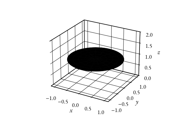
r ⃗ ( u , v ) = ⟨ x ( u , v ) , y ( u , v ) , z ( u , v ) ⟩ . \vec{r}(u, v) = \langle x(u, v), y(u, v), z(u, v) \rangle. r ( u , v ) = ⟨ x ( u , v ) , y ( u , v ) , z ( u , v )⟩ . Example 4 r ⃗ ( u , v ) = ⟨ u cos ( v ) , u sin ( v ) , 1 ⟩ , 0 ≤ u ≤ 1 , 0 ≤ v ≤ 2 π . \vec{r}(u, v) = \langle u \cos(v), u \sin(v), 1 \rangle, \quad 0 \leq u \leq 1, 0 \leq v \leq 2\pi. r ( u , v ) = ⟨ u cos ( v ) , u sin ( v ) , 1 ⟩ , 0 ≤ u ≤ 1 , 0 ≤ v ≤ 2 π . Plotting this parameterization:
Figure 1: The unit disc at height z = 1 z = 1 z = 1 r ⃗ ( u , v ) = ⟨ u cos ( v ) , u sin ( v ) , 1 ⟩ \vec{r}(u, v) = \langle u \cos(v), u \sin(v), 1 \rangle r ( u , v ) = ⟨ u cos ( v ) , u sin ( v ) , 1 ⟩ Example 5 Elliptic paraboloid is the surface with equation:
z = x 2 + 2 y 2 . z = x^2 + 2y^2. z = x 2 + 2 y 2 . The parameterization is therefore:
r ⃗ ( x , y ) = ⟨ x , y , x 2 + 2 y 2 ⟩ . \vec{r}(x, y) = \langle x, y, x^2 + 2y^2 \rangle. r ( x , y ) = ⟨ x , y , x 2 + 2 y 2 ⟩ . Example 6 Find a parameterization of:
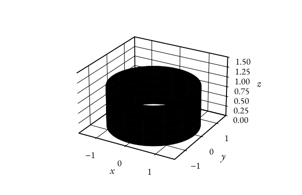
x 2 + y 2 = 2 , 0 ≤ z ≤ 1. x^2 + y^2 = 2, \quad 0 \leq z \leq 1. x 2 + y 2 = 2 , 0 ≤ z ≤ 1. r ⃗ ( u , v ) = ⟨ 2 cos ( u ) , 2 sin ( u ) , v ⟩ , 0 ≤ u ≤ 2 π , 0 ≤ v ≤ 1. \vec{r}(u, v) = \langle \sqrt{2} \cos(u), \sqrt{2} \sin(u), v \rangle, \quad 0 \leq u \leq 2\pi, 0 \leq v \leq 1. r ( u , v ) = ⟨ 2 cos ( u ) , 2 sin ( u ) , v ⟩ , 0 ≤ u ≤ 2 π , 0 ≤ v ≤ 1. Plot:
Figure 2: The cylinder x 2 + y 2 = 2 x^2 + y^2 = 2 x 2 + y 2 = 2 0 ≤ z ≤ 1 0 \leq z \leq 1 0 ≤ z ≤ 1