Signals
Recall (Signal) A signal is a set of information or data. Any physical quantity that varies over time, space or any other variable or variables.
Even, Odd & Periodic
An even function is symmetrical about the vertical axis. Mathematically this means:
f ( t ) = f ( − t ) , f [ k ] = f [ − k ] . f(t) = f(-t), \newline
f[k] = f[-k]. f ( t ) = f ( − t ) , f [ k ] = f [ − k ] . An odd function is anti-symmetrical about the vertical axis. Mathematically this means:
f ( t ) = − f ( − t ) , f [ k ] = − f [ − k ] . f(t) = -f(-t), \newline
f[k] = -f[-k]. f ( t ) = − f ( − t ) , f [ k ] = − f [ − k ] . A periodic function has a fundamental period (minimum), T 0 T_0 T 0 fundamental frequency , f 0 = 1 T 0 f_0 = \dfrac{1}{T_0} f 0 = T 0 1
f ( t ) = f ( t + n T 0 ) , f [ k ] = f [ k + n K 0 ] . f(t) = f(t + nT_0), \newline
f[k] = f[k + nK_0]. f ( t ) = f ( t + n T 0 ) , f [ k ] = f [ k + n K 0 ] . We sometimes define the fundamental frequency in angular velocity instead of Hz, which means, ω 0 = 2 π f 0 = 2 π T 0 \omega_0 = 2\pi f_0 = \dfrac{2\pi}{T_0} ω 0 = 2 π f 0 = T 0 2 π
Convolution
Let’s call our input signal x ( t ) x(t) x ( t ) h ( t ) h(t) h ( t ) y ( t ) y(t) y ( t ) ∗ * ∗
y ( t ) = x ( t ) ∗ h ( t ) . y(t) = x(t) * h(t). y ( t ) = x ( t ) ∗ h ( t ) . The convolution operation is defined as:
y ( t ) = x ( t ) ∗ h ( t ) = ∫ − ∞ + ∞ x ( τ ) h ( t − τ ) d τ . y(t) = x(t) * h(t) = \int_{-\infty}^{+\infty} x(\tau)h(t - \tau) \, d\tau. y ( t ) = x ( t ) ∗ h ( t ) = ∫ − ∞ + ∞ x ( τ ) h ( t − τ ) d τ . In the discrete case:
c [ k ] = f [ k ] ∗ g [ k ] = ∑ m = − ∞ + ∞ f [ m ] g [ k − m ] . c[k] = f[k] * g[k] = \sum_{m = -\infty}^{+\infty} f[m]g[k - m]. c [ k ] = f [ k ] ∗ g [ k ] = m = − ∞ ∑ + ∞ f [ m ] g [ k − m ] . This operation is also:
Commutative:
f 1 ( t ) ∗ f 2 ( t ) = f 2 ( t ) ∗ f 1 ( t ) . f_1(t) * f_2(t) = f_2(t) * f_1(t). f 1 ( t ) ∗ f 2 ( t ) = f 2 ( t ) ∗ f 1 ( t ) . Distributive:
f 1 ( t ) ∗ ( f 2 ( t ) + f 3 ( t ) ) = f 1 ( t ) ∗ f 2 ( t ) + f 1 ( t ) ∗ f 3 ( t ) . f_1(t) * (f_2(t) + f_3(t)) = f_1(t) * f_2(t) + f_1(t) * f_3(t). f 1 ( t ) ∗ ( f 2 ( t ) + f 3 ( t )) = f 1 ( t ) ∗ f 2 ( t ) + f 1 ( t ) ∗ f 3 ( t ) . Associative:
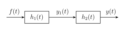
f 1 ( t ) ∗ ( f 2 ( t ) ∗ f 3 ( t ) ) = ( f 1 ( t ) ∗ f 2 ( t ) ) ∗ f 3 ( t ) . f_1(t) * (f_2(t) * f_3(t)) = (f_1(t) * f_2(t)) * f_3(t). f 1 ( t ) ∗ ( f 2 ( t ) ∗ f 3 ( t )) = ( f 1 ( t ) ∗ f 2 ( t )) ∗ f 3 ( t ) . Figure 1: Two systems h 1 ( t ) h_1(t) h 1 ( t ) h 2 ( t ) h_2(t) h 2 ( t ) Using these properties we can say that:
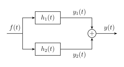
y ( t ) = f ( t ) ∗ h ( t ) , h ( t ) = h 1 ( t ) ∗ h 2 ( t ) . y(t) = f(t) * h(t), \quad h(t) = h_1(t) * h_2(t). y ( t ) = f ( t ) ∗ h ( t ) , h ( t ) = h 1 ( t ) ∗ h 2 ( t ) . In the parallel case:
Figure 2: Two systems h 1 ( t ) h_1(t) h 1 ( t ) h 2 ( t ) h_2(t) h 2 ( t ) f ( t ) ∗ h ( t ) , h ( t ) = h 1 ( t ) + h 2 ( t ) . f(t) * h(t), \quad h(t) = h_1(t) + h_2(t). f ( t ) ∗ h ( t ) , h ( t ) = h 1 ( t ) + h 2 ( t ) . Shift:
f 1 ( t ) ∗ f 2 ( t ) = c ( t ) , f 1 ( t ) ∗ f 2 ( t − T ) = c ( t − T ) , f 1 ( t − T ) ∗ f 2 ( t ) = c ( t − T ) , f 1 ( t − T 1 ) ∗ f 2 ( t − T 2 ) = c ( t − T 1 − T 2 ) . \begin{align*}
f_1(t) * f_2(t) & = c(t), \newline
f_1(t) * f_2(t - T) & = c(t - T), \newline
f_1(t - T) * f_2(t) & = c(t - T), \newline
f_1(t - T_1) * f_2(t - T_2) & = c(t - T_1 - T_2).
\end{align*} f 1 ( t ) ∗ f 2 ( t ) f 1 ( t ) ∗ f 2 ( t − T ) f 1 ( t − T ) ∗ f 2 ( t ) f 1 ( t − T 1 ) ∗ f 2 ( t − T 2 ) = c ( t ) , = c ( t − T ) , = c ( t − T ) , = c ( t − T 1 − T 2 ) . Convolution with an impulse:
f ( t ) ∗ δ ( t ) = f ( t ) . f(t) * \delta(t) = f(t). f ( t ) ∗ δ ( t ) = f ( t ) . We can combine these two:
Convolution with an impulse:
f ( t ) ∗ δ ( t − T ) = f ( t − T ) . f(t) * \delta(t - T) = f(t - T). f ( t ) ∗ δ ( t − T ) = f ( t − T ) . Differential Equations in the time-domain
As we defined, the output of these systems are the result of two independent cases.
So for the zero-input response:
Q ( D ) y 0 ( t ) = 0. Q(D)y_0(t) = 0. Q ( D ) y 0 ( t ) = 0. The solution for y 0 ( t ) y_0(t) y 0 ( t )
y 0 ( t ) = c 1 e λ 1 t + c 2 e λ 2 t + … + c n e λ n t . y_0(t) = c_1 e^{\lambda_1 t} + c_2 e^{\lambda_2 t} + \ldots + c_n e^{\lambda_n t}. y 0 ( t ) = c 1 e λ 1 t + c 2 e λ 2 t + … + c n e λ n t . If repeated roots:
y 0 ( t ) = ( c 1 + c 2 t + … + c r t r − 1 ) e λ 1 t + c r + 1 e λ r + 1 t + … + c n e λ n t . y_0(t) = (c_1 + c_2t + \ldots + c_r t^{r - 1})e^{\lambda_1 t} + c_{r + 1}e^{\lambda_{r + 1} t} + \ldots + c_n e^{\lambda_n t}. y 0 ( t ) = ( c 1 + c 2 t + … + c r t r − 1 ) e λ 1 t + c r + 1 e λ r + 1 t + … + c n e λ n t . Also in the case we have complex roots, α ± j β \alpha \pm j \beta α ± j β
y 0 ( t ) = c 2 e j θ e ( α + j β ) t + c 2 e − j θ e ( α − j β ) t = c 2 e α t [ e j ( β t + θ ) + e − j ( β t + θ ) ] . y_0(t) = \dfrac{c}{2} e^{j \theta} e^{(\alpha + j \beta)t} + \dfrac{c}{2} e^{-j \theta} e^{(\alpha - j \beta)t} = \dfrac{c}{2} e^{\alpha t} \left[ e^{j(\beta t + \theta)} + e^{-j(\beta t + \theta)}\right]. y 0 ( t ) = 2 c e j θ e ( α + j β ) t + 2 c e − j θ e ( α − j β ) t = 2 c e α t [ e j ( β t + θ ) + e − j ( β t + θ ) ] . Using Euler’s formula:
y 0 ( t ) = c e α t cos ( β t + θ ) . y_0(t) = c e^{\alpha t} \cos(\beta t + \theta). y 0 ( t ) = c e α t cos ( β t + θ ) . Example 1 ( D 2 + 3 D + 2 ) y 0 ( t ) = 0 , (D^2 + 3D + 2)y_0(t) = 0, ( D 2 + 3 D + 2 ) y 0 ( t ) = 0 , λ 2 + 3 λ + 2 = ( λ + 1 ) ( λ + 2 ) = 0 , \lambda^2 + 3\lambda + 2 = (\lambda + 1)(\lambda + 2) = 0, λ 2 + 3 λ + 2 = ( λ + 1 ) ( λ + 2 ) = 0 , λ 1 = − 1 , λ 2 = − 2 , \lambda_1 = -1, \quad \lambda_2 = -2, λ 1 = − 1 , λ 2 = − 2 , y 0 ( t ) = c 1 e − t + c 2 e − 2 t . y_0(t) = c_1 e^{-t} + c_2 e^{-2t}. y 0 ( t ) = c 1 e − t + c 2 e − 2 t . Trigonometric Fourier series
ω 0 \omega_0 ω 0
n ω 0 n \omega_0 n ω 0 n n n
We can call the fundamental period for, T 0 T_0 T 0
T 0 = 2 π ω 0 . T_0 = \dfrac{2\pi}{\omega_0}. T 0 = ω 0 2 π . So:
f ( t ) = a 0 + a 1 cos ω 0 t + a 2 cos 2 ω 0 t + b 1 sin ω 0 t + b 2 sin 2 ω 0 t + … f(t) = a_0 + a_1 \cos \omega_0 t + a_2 \cos 2\omega_0 t + b_1 \sin \omega_0 t + b_2 \sin 2\omega_0 t + \ldots f ( t ) = a 0 + a 1 cos ω 0 t + a 2 cos 2 ω 0 t + b 1 sin ω 0 t + b 2 sin 2 ω 0 t + … We can write this more compactly.
a n cos n ω 0 t + b n sin n ω 0 t = C n cos ( n ω 0 t + θ n ) . a_n \cos n\omega_0 t + b_n \sin n\omega_0 t = C_n \cos(n\omega_0 t + \theta_n). a n cos n ω 0 t + b n sin n ω 0 t = C n cos ( n ω 0 t + θ n ) . Where:
C n = a n 2 + b n 2 , C_n = \sqrt{a_n^2 + b_n^2}, C n = a n 2 + b n 2 , θ n = tan − 1 ( − b n a n ) . \theta_n = \tan^{-1} \left(\dfrac{-b_n}{a_n}\right). θ n = tan − 1 ( a n − b n ) . So:
f ( t ) = C 0 + ∑ n = 1 ∞ C n cos ( n ω 0 t + θ n ) . f(t) = C_0 + \sum_{n = 1}^{\infty} C_n \cos(n\omega_0 t + \theta_n). f ( t ) = C 0 + n = 1 ∑ ∞ C n cos ( n ω 0 t + θ n ) . Exponential Fourier series
f ( t ) = ∑ n = − ∞ ∞ D n e j n ω 0 t . f(t) = \sum_{n = -\infty}^{\infty} D_n e^{jn\omega_0 t}. f ( t ) = n = − ∞ ∑ ∞ D n e j n ω 0 t . C n cos ( n ω 0 t + θ n ) = C n 2 ( e j ( n ω 0 t + θ n ) + e − j ( n ω 0 t + θ n ) ) = ( C n 2 e j θ n ) e j n ω 0 t + ( C n 2 e − j θ n ) e − j n ω 0 t . \begin{align*}
C_n \cos(n\omega_0 t + \theta_n) & = \dfrac{C_n}{2} \left(e^{j(n\omega_0 t + \theta_n)} + e^{-j(n\omega_0 t + \theta_n)}\right) \newline
& = \left(\dfrac{C_n}{2} e^{j\theta_n}\right) e^{jn\omega_0 t} + \left(\dfrac{C_n}{2} e^{-j\theta_n}\right) e^{-jn\omega_0 t}.
\end{align*} C n cos ( n ω 0 t + θ n ) = 2 C n ( e j ( n ω 0 t + θ n ) + e − j ( n ω 0 t + θ n ) ) = ( 2 C n e j θ n ) e j n ω 0 t + ( 2 C n e − j θ n ) e − j n ω 0 t . D n = 1 2 C n e j θ n , D_n = \dfrac{1}{2} C_n e^{j\theta_n}, D n = 2 1 C n e j θ n , D − n = 1 2 C n e − j θ n , D_{-n} = \dfrac{1}{2} C_n e^{-j\theta_n}, D − n = 2 1 C n e − j θ n , f ( t ) = D 0 + ∑ n = 1 ∞ ( D n e j n ω 0 t + D − n e − j n ω 0 t ) , f(t) = D_0 + \sum_{n = 1}^{\infty} (D_n e^{jn\omega_0 t} + D_{-n} e^{-jn\omega_0 t}), f ( t ) = D 0 + n = 1 ∑ ∞ ( D n e j n ω 0 t + D − n e − j n ω 0 t ) , f ( t ) = ∑ n = − ∞ ∞ D n e j n ω 0 t . f(t) = \sum_{n = -\infty}^{\infty} D_n e^{jn\omega_0 t}. f ( t ) = n = − ∞ ∑ ∞ D n e j n ω 0 t . Recall (Fourier transform) F ( ω ) = ∫ − ∞ ∞ f ( t ) e − j ω t d t , F(\omega) = \int_{-\infty}^{\infty} f(t) e^{-j\omega t} \, dt, F ( ω ) = ∫ − ∞ ∞ f ( t ) e − j ω t d t , f ( t ) = 1 2 π ∫ − ∞ ∞ F ( ω ) e j ω t d ω , f(t) = \dfrac{1}{2\pi} \int_{-\infty}^{\infty} F(\omega) e^{j\omega t} \, d\omega, f ( t ) = 2 π 1 ∫ − ∞ ∞ F ( ω ) e j ω t d ω , f ( t ) ⟺ F ( ω ) . f(t) \iff F(\omega). f ( t ) ⟺ F ( ω ) . Example 2 f ( t ) = rect ( t τ ) , f(t) = \operatorname{rect}\left(\dfrac{t}{\tau}\right), f ( t ) = rect ( τ t ) , F ( ω ) = ∫ − ∞ ∞ rect ( t τ ) e − j ω t d t = ∫ − τ 2 τ 2 e − j ω t d t = − 1 j ω e − j ω t ∣ − τ 2 τ 2 = − 1 j ω ( e − j ω τ 2 − e j ω τ 2 ) = 2 sin ( ω τ 2 ) ω = τ sin ( ω τ 2 ) ω τ 2 = τ sinc ( ω τ 2 ) , \begin{align*}
F(\omega) & = \int_{-\infty}^{\infty} \operatorname{rect}\left(\dfrac{t}{\tau}\right) e^{-j\omega t} \, dt \newline
& = \int_{-\frac{\tau}{2}}^{\frac{\tau}{2}} e^{-j\omega t} \, dt \newline
& = -\dfrac{1}{j\omega} e^{-j\omega t} \bigg\rvert_{-\frac{\tau}{2}}^{\frac{\tau}{2}} \newline
& = -\dfrac{1}{j\omega} \left(e^{-j\omega \frac{\tau}{2}} - e^{j\omega \frac{\tau}{2}}\right) \newline
& = \dfrac{2 \sin\left(\dfrac{\omega \tau}{2}\right)}{\omega} \newline
& = \tau \dfrac{\sin\left(\dfrac{\omega \tau}{2}\right)}{\dfrac{\omega \tau}{2}} \newline
& = \tau \operatorname{sinc}\left(\dfrac{\omega \tau}{2}\right),
\end{align*} F ( ω ) = ∫ − ∞ ∞ rect ( τ t ) e − j ω t d t = ∫ − 2 τ 2 τ e − j ω t d t = − j ω 1 e − j ω t − 2 τ 2 τ = − j ω 1 ( e − j ω 2 τ − e j ω 2 τ ) = ω 2 sin ( 2 ω τ ) = τ 2 ω τ sin ( 2 ω τ ) = τ sinc ( 2 ω τ ) , rect ( t τ ) ⟺ τ sinc ( ω τ 2 ) . \operatorname{rect}\left(\dfrac{t}{\tau}\right) \iff \tau \operatorname{sinc}\left(\dfrac{\omega \tau}{2}\right). rect ( τ t ) ⟺ τ sinc ( 2 ω τ ) . Transfer function
Say we have a system which can be modeled as:
y ( t ) = f ( t ) ∗ h ( t ) . y(t) = f(t) * h(t). y ( t ) = f ( t ) ∗ h ( t ) . The same system, but in the frequency domain is therefore:
Y ( ω ) = F ( ω ) H ( ω ) . Y(\omega) = F(\omega) H(\omega). Y ( ω ) = F ( ω ) H ( ω ) . Just as we call, h ( t ) h(t) h ( t ) H ( ω ) H(\omega) H ( ω )
Since, in the most general case, we view our frequency functions as complex functions. We can say that
An input signal’s spectral component of frequency, ω \omega ω ∣ H ( ω ) ∣ |H(\omega)| ∣ H ( ω ) ∣ ∠ H ( ω ) \angle H(\omega) ∠ H ( ω )
However, since we modify the phase, this means that our output signal may have a different waveform than our input.
Recall (Nyquist-Shannon sampling theorem) A real signal whose bandwidth is limited to B B B F s > 2 B \mathcal{F}_s > 2B F s > 2 B
Recall (Laplace transform) The Laplace transformation is a unilateral transform , which just means it is one-sided.
Given a function that is defined for t ≥ 0 t \geq 0 t ≥ 0 [ 0 , ∞ ) [0, \infty) [ 0 , ∞ )
F ( s ) = L [ f ( t ) ] = ∫ 0 ∞ f ( t ) e − s t d t . F(s) = \mathcal{L}[f(t)] = \int_0^{\infty} f(t)e^{-st} \, dt. F ( s ) = L [ f ( t )] = ∫ 0 ∞ f ( t ) e − s t d t .