Part 3 - 2nd Law of Thermodynamics

In this part we’ll cover the 2nd law of thermodynamics - as well as summarize this field of physics.

Direction for $W$ and $Q$

As we’ve seen, the work $W$ and $Q$ are quite important. So let’s set up some general guide lines.

Generally, in a given thermal system:

An expansion, $V_f > V_i \rightarrow W > 0$
A compression, $V_f < V_i \rightarrow W < 0$
Increase in temperature, $\Delta T > 0 \ (T_f > T_i) \rightarrow Q > 0$
Decrease in temperature, $\Delta T < 0 \ (T_f < T_i) \rightarrow Q < 0$

Sometimes it can be quite tricky to know if the temperature increases or decreases - but there’s a general rule for that as well.

Since we have $PV = nRT$ , the farther away you are from the origin, the higher the temperature.

But we can always use $PV = nRT$ and see what kind of change we have in $T$ .

Directions of the Different Processes

Now that we have a general understanding of directions, let’s go back to our 4 different processes and see what directions they have.

Isobaric Process

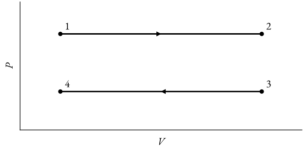
Here’s a plot of an isobar process - with two different directions.

In the above case, the gas increases in volume - therefore it has done a positive work. Using $PV = nRT$ we can see that $T$ has to increase since $P$ stays constant.

In the other case, it’s just the opposite, we decrease in $V$ therefore a negative work has been done - same reasoning as before, since $P$ is constant $T$ has to decrease as well.

\begin{align*} W_{12} & > 0, & Q_{12} & > 0, \newline W_{34} & < 0, & Q_{34} & < 0. \end{align*}

Isochoric Process

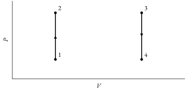
Here’s a plot of an isochoric process - with two different directions.

As we can see, no work is being done by either of the processes. But we can say something about the temperature and $Q$ .

In the case we increase in pressure, it also means $T$ increases. Same logic goes for when $P$ decreases, $T$ decreases.

\begin{align*} W_{12} & = 0, & Q_{12} & > 0, \newline W_{34} & = 0, & Q_{34} & < 0. \end{align*}

Isothermal Process

The isothermal process is a bit more tricky, but it becomes,

\begin{align*} \text{Positive direction:} & \quad W_{12} > 0, & Q_{12} & > 0, \newline \text{Negative direction:} & \quad W_{34} < 0, & Q_{34} & < 0. \end{align*}

Adiabatic Process

In an adiabatic process, $Q = 0$ therefore it becomes,

\begin{align*} \text{Positive direction:} & \quad W_{12} > 0, & Q_{12} & = 0, \newline \text{Negative direction:} & \quad W_{34} < 0, & Q_{34} & = 0. \end{align*}

The Carnot Cycle

The Carnot cycle is a famous thermodynamic cycle since it’s the ‘upper-limit’ of any thermodynamic engine that transfers heat into work. The proof of the Carnot cycle’s efficiency is quite a long and complicated one so I’m not going to prove it but - the efficiency of a ‘Carnot machine’ would be,

e = \frac{T_h - T_c}{T_h},

or generally written as,

e = 1 - \frac{T_c}{T_h}.

The Reverse Carnot Cycle

Instead of using heat to perform work - we might want to cool something down or just transfer heat from one place to another. Then the efficiency doesn’t tell us much.

Instead we look at something called coefficient of performance.

For a refrigeration cycle,

K = \frac{Q_{\text{in}}}{Q_{\text{out}} - Q_{\text{in}}} = \frac{T_c}{T_h - T_c}.

For a heat pump,

K = \frac{Q_{\text{out}}}{Q_{\text{out}} - Q_{\text{in}}} = \frac{T_h}{T_h - T_c}.

Thermodynamics 2nd Law

Before we formally define the 2nd law - we first need to refresh our memory of what entropy and exergy are. Very briefly, we can explain entropy as how ‘unorganized’ a substance is. Exergy could be defined as the quality of energy, for example.

It takes $\approx 300\,000 \ \mathrm{J}$ of energy to heat 1 kg of $0^{\circ}\mathrm{C}$ water to $70^{\circ}\mathrm{C}$ . If we could transfer all of this energy to kinetic energy, the water could have a speed of $\approx 770 \ \mathrm{m/s}$ - but as we know, it’s not possible.

But alright, time to formally define the 2nd law,

Theorem 1 (2nd law of thermodynamics)

dS = \frac{dQ}{T}, \quad dS_{\text{system}} \geq 0

Combining 1st and 2nd Law

If we combine the 1st and the new 2nd law - we will get,

dU = T \, dS - P \, dV.

So now we can utilize something called $TS$ diagrams instead of always using $PV$ diagrams. In $TS$ diagrams it’s really easy to calculate $Q$ .

Conclusion

This concludes this part and the series as a whole (probably). I really enjoyed writing and will probably continue writing all my notes here, since I learn a lot doing this.