Let’s call this last expression for ℓ(θ), this is a lower bound of the original objective L(θ).
The equality holds when q(z(i))p(x(i),z(i);θ) is a constant.
This can be achieved for q(z(i))=p(z(i)∣x(i);θ).
The EM algorithm aims to optimize the lower bound ℓ(θ),
By definition, this is the (log) likelihood of the data.
By marginalization over z(i) and multiplication of an arbitrary distribution q(z(i)) to both numerator and denominator inside log.
By Jensen’s inequality where equality condition is satisfied by setting q(t)(z(i))=p(z(i)∣x(i);θ(t)).
By M-step of EM, where we maximize (3), holding q(t)(z(i)) fixed.
By Jensen’s inequality (in reverse order). Note that we have already updated θ from θ(t) to θ(t+1), q(t)(z(i)) may now not satisfy the equality condition.
By definition, this is the lower bound of the likelihood.
Hence, EM causes the likelihood to increase monotonically.
Remark
Note (EM as coordinate ascent)
One remark that we have to do is, if we define the EM as,
We can view this as coordinate ascent on J, in which the E-step maximizes J with respect to q, and the M-step maximizes J with respect to θ.
One can easily prove this using Lagrangian multipliers!
Clustering Summary
Clustering Task
Given a set of input vectors D={x(i)}i=1M, with x(i)∈RN, group similar x(i) into clusters.
Estimate a cluster center, representing the data points in that cluster.
Predict the cluster for a new data point.
Exhaustive clustering
Cluster shape: Arbitrary shape.
Principle: Minimize an assumed clustering criterion with brute-force search.
Pros: Optimal under the given clustering criterion.
Cons: Impractical to construct the clustering criterion, prohibitive to compute.
K-means
Cluster shape: Circular.
Principle: Minimize distance to cluster center.
Pros: Simple and scalable (MiniBatchKMeans).
Cons: Sensitive to initialization, could get bad solutions due to local minima, need to choose K.
Gaussian Mixture Model (GMM)
Cluster shape: Elliptical.
Principle: Maximum likelihood using expectation maximization.
Pros: Elliptical cluster shapes.
Cons: Sensitive to initialization, could get bad solutions due to local minima, need to choose K.
Feature normalization
Feature normalization is typically required for clustering.
E.g., algorithms based on Euclidean distance (K-means).
Dimensionality Reduction
Transform high-dimensional vectors into low-dimensional vectors.
Dimensions in the low-dimensional data represent co-occurring features in the high-dimensional data.
Dimensions in the low-dimensional data may have semantic meaning.
For example, in document analysis.
High-dimensional data: Bag-of-word vectors of documents.
Low-dimensional data: Each dimension represents similarity to a topic.
Reasons for Dimensionality Reduction
Preprocessing, makes the dataset easier to use.
Reduce computational cost of running machine learning algorithms.
Can be used to “de-noise” data by projecting to lower-dimensional space and then projecting back to the original high-dimensional space.
Makes the results easier to understand (e.g., visualization).
Dimensionality Reduction VS. Feature Selection
The goal of feature selection is to remove features that are not informative with respect to the class label.
This obviously reduces the dimensionality of the feature space.
Dimensionality reduction can be used to find a meaningful lower-dimensional feature space even when there is information in each feature dimension so that none can be discarded.
Another important property of dimensionality reduction is that it is unsupervised.
While dimensionality reduction can be seen as a simplistic form of (data) compression, it is not equivalent to it, as the goal of compression is to reduce the expected code length (which is lower bounded by entropy) of the representation not only the dimensionality.
For example, in lossless compression, arithmetic coding encodes the entire data into a single number, an arbitrary-precision fraction q where 0.0≤q<1.0.
Linear Dimensionality Reduction
In linear dimensionality reduction we project the original data onto a lower-dimensional hyperplane (e.g., line, plane).
I.e., move and rotate the coordinate axis of the data, then we represent the data with coordinates in the new component space.
Mathematically, this can be written as,
x(i)=k=1∑Kzk(i)bk,
where bk is a basis vector and zk(i)∈R is the corresponding weight.
Connection to Linear Regression
If we focus on the j-th entry of x(i), we have,
xj(i)=k=1∑Kzk(i)bjk.
This expression can be seen as linear regression.
xj(i) is the target.
zk(i) for each k are the weights.
bjk for each k are the features.
Alternatively, we may view zk(i) as feature and bjk as weights.
Unlike linear regression, we only know “targets”. We must learn both features and weights.
Matrix Formulation
Let X∈RM×N be the data matrix, with one data case x(i)∈RN per row.
X=−−−−−−(x(1))T(x(2))T⋮(x(M))T−−−−−−.
Let Z∈RM×K be the loading matrix and B∈RK×N be the factor matrix.
However, most real world data will be subject to noise.
If we assume that ϵ∈RM×N is a matrix of noise values from some probability distribution, we have,
X=ZB+ϵ.
Learning Criterion
The learning problem for linear dimensionality reduction is to estimate values for both Z and B given only the noisy observations of X.
One possible learning criterion is to minimize the sum of squared errors when reconstructingX from Z and B.
This leads to,
Z,Bargmin∥X−ZB∥F2,
Where ∥⋅∥F is the Frobenius norm of a matrix, defined as,
∥A∥F=ij∑Aij2.
Alternating Least Squares
By leveraging the OLS solution for linear regression, we can estimate Z and B using Alternating Least Squares (ALS).
Starting from some random initialization, ALS iterates between two steps until convergence.
Algorithm 2: Alternating least squares
Assume Z is fixed and optimize B,
B←(ZTZ)−1ZTX.
Assume B is fixed and optimize Z,
ZT←(BBT)−1BXT.
Lack of Uniqueness for Optimal Parameters
Suppose we run the ALS algorithm to convergence and obtain optimal parameters Z⋆ and B⋆ such that,
ℓ⋆=∥X−Z⋆B⋆∥F2.
Let R∈RK×K be an arbitrary invertible matrix.
A K×K matrix R is invertible, if there exists a K×K matrix S such that RS=SR=I.
Which we also can denote as R−1=S.
We obtain a different set of parameters Z~=Z⋆R and B~=R−1B⋆, with the same optimal value,
ℓ⋆=∥X−Z⋆(I)B⋆∥F2=∥X−Z⋆(RR−1)B⋆∥F2=∥X−Z~B~∥F2.
We can obtain the global optimal solution(s) and make them unique by specifying additional criteria.
Singular Value Decomposition (SVD)
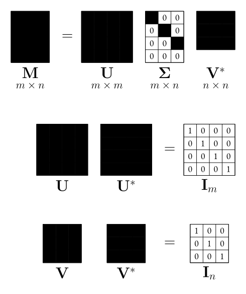
Let X be an M×N matrix, with M≥N. It can be factorized as,
X=U(Σ0)VT,
Where U∈RM×M and V∈RN×N are orthogonal, i.e.,
UTU=UUT=IM,VTV=VVT=IN.
Columns of U and V are called left and right singular vectors of X, respectively.
Σ∈RM×N is a diagonal matrix,
Σ=diag(σ1,σ2,…,σN),σ1≥σ2≥…≥σN≥0.
σi’s are called singular values of X.
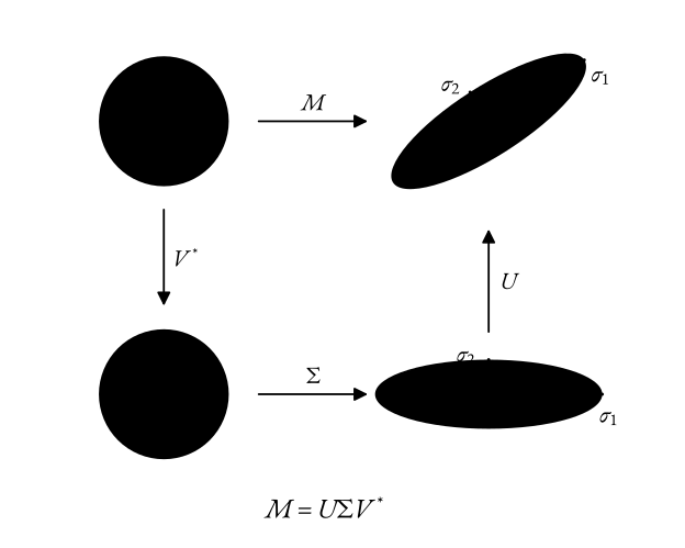
Figure 1: SVD visualization of the matrices.Figure 2: SVD visualization of the different operations.
Upper Left: The unit disc with the two canonical unit vectors.
Upper Right: Transformed with M.
Lower Left: The action of VT. This is just a rotation.
Lower Right: The action of ΣVT. Σ scales vertically and horizontally.
Reduced-Form SVD
If only K<min{M,N} singular values are non-zero, the SVD X∈RM×N can be represented in reduced form as follows,
X=UΣKVT,
which we can write as,
X=k=1∑KσkukvkT.
Where
U=[u1,u2,…,uK]∈RM×K.
UTU=IK.
V=[v1,v2,…,vK]∈RN×K.
VTV=IK.
ΣK=diag(σ1,σ2,…,σK)∈RK×K.
σ1≥σ2≥…≥σK≥0.
ukvkT∈RM×N is the product of a column vector uk and a row vector vkT.
It has rank 1.
X is a weighted summation of K rank-1 matrices.
Eckart-Young-Mirsky Theorem
Theorem 2 (Eckart-Young-Mirsky Theorem)
Given an M×N matrix X of rank R≤min{M,N} and its singular value decomposition X=UΣRVT
with singular values σ1≥σ2≥…≥σR>0 and the rest being zero,
then among all M×N matrices of lower rank K≤R,
the best approximation is Y⋆=UΣKVT, where ΣK is the diagonal matrix with singular values σ1,σ2,…,σK in the sense that 2,
∥X−Y⋆∥F2=min{∥X−Y∥F2∣Y∈RM×N,rankY≤K}.
SVD provides a unique solution to minimum Frobenius norm linear dimensionality reduction.
References
Arthur P. Dempster, Nan M. Laird, and Donald B. Rubin (1977) “Maximum Likelihood from Incomplete Data via the EM Algorithm”. Journal of the Royal Statistical Society: Series B 39, 1-38. Link
Carl Eckart and Gale Young (1936) “The Approximation of One Matrix by Another of Lower Rank”. Psychometrika 1, 211-218. Link