Part 6 - Graphical Models I

Introduction

In this part, we will introduce Bayesian networks, which are probabilistic graphical models that represent a set of variables and their conditional dependencies via a directed acyclic graph (DAG). Bayesian networks are powerful tools for modeling complex systems and reasoning under uncertainty. We will discuss some fundamental theory and their applications.

Graphical Models

Intuition (Graphical Models)

Graphical models are a powerful framework to represent and learn structured probability models.

The main idea behind graphical models is that they capture a way in which a joint distribution can be factorized into product of factors, each depending only on a subset of variables. They are generally useful for, visualizing the structure of a probabilistic model, encoding structural information (i.e., dependencies) about involved random variables, and provide structure in computations, i.e., provide graph-based algorithms for computations, inference, and prediction.

There are three main types of graphical models,

Bayesian Networks (or Bayes nets) which are DAGs 11Directed Acyclic Graphs (DAGs) are graphs with directed edges and no cycles.. They represent a set of random variables and their conditional dependence structure.
Markov Random Fields which are undirected graphs. They represent a set of random variables and their Markov structure (i.e., conditional independence structure).
Factor Graphs. Which are more convenient for the purposes of inference and learning.

Bayesian Networks

Definition 1 (Bayesian Networks)

In a Bayesian network, we have two types of elements.

Nodes represents the random variables and more specifically, an empty node is an unobserved variable, while a shaded node is an observed variable.
Edges represents the relationships between the random variables.

Further, the bayesian netowrk encodes a factorization of a join distribution.

Assume we have $K$ random variables $\{\mathsf{x}_1, \mathsf{x}_2, \ldots, \mathsf{x}_K\}$ with join probability distribution $p(\mathsf{x}_1, \mathsf{x}_2, \ldots, \mathsf{x}_K)$ , we know by the chain rule of probability that,

\begin{align*} p(\mathsf{x}_1, \mathsf{x}_2, \ldots, \mathsf{x}_K) & = p(\mathsf{x}_1) p(\mathsf{x}_2 \mid \mathsf{x}_1) p(\mathsf{x}_3 \mid \mathsf{x}_1, \mathsf{x}_2) \cdots p(\mathsf{x}_K \mid \mathsf{x}_1, \mathsf{x}_2, \ldots, \mathsf{x}_{K-1}) \newline & = \prod_{i=1}^{K} p(\mathsf{x}_i \mid p(\mathsf{x}_i)) \newline \end{align*}

To build a Bayesian network we need,

Introduce a node for each $\mathsf{x}$ and associate the node with $p(\mathsf{x} \mid \cdot)$ .
For each $p(\mathsf{x} \mid \cdot)$ , draw a directed edge to node $\mathsf{x}$ from nodes corresponding to RVs on which the distribution is conditioned.
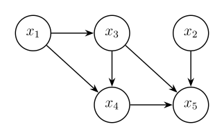
Edge from node $\mathsf{x}$ to node $\tilde{\mathsf{x}}$ , $\mathsf{x}$ parent of $\tilde{\mathsf{x}}$ , $\tilde{\mathsf{x}}$ child of $\mathsf{x}$ .

Example 1 (Bayesian Network Example)

Consider the network in Figure 1, the corresponding joint distribution is given by,

p(x_1, x_2, x_3, x_4, x_5) = p(x_1) p(x_2) p(x_3 \mid x_1) p(x_4 \mid x_1, x_3) p(x_5 \mid x_2, x_3, x_4)

Definition 2 (Bayesian Networks (Continued))

A Bayesian network is a directed acyclic graph (DAG) whose nodes represents random variables $\{\mathsf{x}_1, \mathsf{x}_2, \ldots, \mathsf{x}_K\}$ with an associated joint distribution that factorizes as,

p(\mathsf{x}_1, \mathsf{x}_2, \ldots, \mathsf{x}_K) = \prod_{k = 1}^{K} p(\mathsf{x}_k \mid \mathsf{x}_{\mathcal{P}(\mathsf{x}_k)}),

where $\mathcal{P}(\mathsf{x}_k)$ denotes the set of parents of node $\mathsf{x}_k$ in the graph.

Note

Note that $\mathsf{x}_{\mathcal{P}(\mathsf{x}_k)}$ accounts for statistical dependence of $\mathsf{x}_k$ with all the preceding variables $\{\mathsf{x}_1, \ldots, \mathsf{x}_{k-1}\}$ according to selected order. The corresponding Bayesian network encodes,

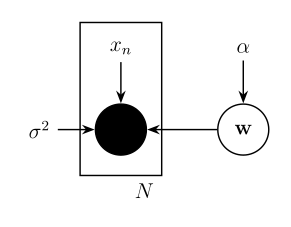
\mathsf{x}_k \perp \{\mathsf{x}_1, \ldots, \mathsf{x}_{k-1}\} \setminus \mathcal{P}(\mathsf{x}_k) \mid \mathsf{x}_{\mathcal{P}(\mathsf{x}_k)}

Example 2 (Bayesian Polynomial Regression)

Consider the joint distribution condtioned on input data and model parameters,

p(y_{\mathcal{D}}, \mathbf{w} \mid x_{\mathcal{D}}, \alpha, \sigma^2) = p(\mathbf{w} \mid \alpha) \prod_{i=1}^{N} p(y_i \mid \mathbf{x}_i, \mathbf{w}, \sigma^2)

Causal Relationships

Intuition (Causal Relationships)

Bayesian networks are especially useful for modeling causal relationships between variables.

If we can identify causal relationships among random variables, this must mean there is a natural order on variables, i.e., random variables that appear later caused by a subset of preceding variables.

Causing random variables for random variable $\mathsf{x}_k$ are included in $\mathcal{P}(\mathsf{x}_k)$ . Which means conditioning on $\mathsf{x}_{\mathcal{P}(\mathsf{x}_k)}$ , $\mathsf{x}_k$ is independent of all other preceding variables.

Intuition (Ancestral Sampling)

However, we usually have a problem when dealing with causal relationships, i.e., obtaining marginals is not a trivial task.

But we can approximate exact distribution by an empirical one built from samples and perfect task for Bayesian networks.

Algorithm (Ancestral Sampling)

Assume,

p(\mathsf{x}_1, \mathsf{x}_2, \ldots, \mathsf{x}_K) = \prod_{k = 1}^{K} p(\mathsf{x}_k \mid \mathsf{x}_{\mathcal{P}(\mathsf{x}_k)}),

i.e., ordered variables $\{\mathsf{x}_1, \mathsf{x}_2, \ldots, \mathsf{x}_K\}$ , with no arrow from any node to any lower numbered node.

Draw sample for $\mathsf{x}_1$ from $p(\mathsf{x}_1)$ .
Draw sample for $\mathsf{x}_2$ from $p(\mathsf{x}_2 \mid \mathsf{x}_1)$ .
$\ldots$
Draw sample for $\mathsf{x}_K$ from $p(\mathsf{x}_K \mid \mathsf{x}_{\mathcal{P}(\mathsf{x}_K)})$ .

Thus, we have obtained a sample from the joint distribution.

To sample from a marginal distribution we,

Take sampled values for required nodes and ignore those remaining ones.
$p(\mathsf{x}_2, \mathsf{x}_4)$ : sample from $p(\mathsf{x}_1, \ldots, \mathsf{x}_K)$ , retain $\hat{\mathsf{x}}_2$ and $\hat{\mathsf{x}}_4$ and discard $\{\hat{\mathsf{x}}_{j \neq 2,4}\}$ .

Definition 3 (Conditional Independence)

We know from classical probability theory that two random variables $a$ and $b$ are conditionally independent given a third random variable $c$ if,

p(a, b \mid c) = p(a \mid c) p(b \mid c)

When dealing with graphical models, we denote conditional independence as,

a \perp b \mid c

This can also be written as,

p(a \mid b, c) = \frac{p(a, b, c)}{p(b, c)} = \frac{p(a, b \mid c)}{p(b \mid c)} = \frac{p(a \mid c) p(b \mid c)}{p(b \mid c)} = p(a \mid c)

The three basic structures for conditional independence

Intuition (Types of Connections)

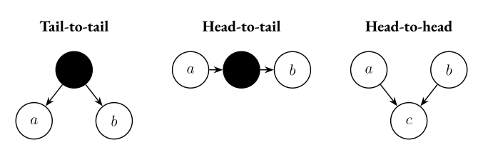
Observe Figure 3, in the case of a tail-to-tail connection,

p(a, b \mid c) = \frac{p(a, b, c)}{p(c)} = \frac{p(a \mid c) p(b \mid c) p(c)}{p(c)} = p(a \mid c) p(b \mid c) \implies a \perp b \mid c

i.e., $a$ and $b$ are independent if node in between is observed.

In the case of a head-to-tail connection,

p(a, b \mid c) = \frac{p(a, b, c)}{p(c)} = \frac{p(a) p(c \mid a) p(b \mid c)}{p(c)} = p(a \mid c) p(b \mid c) \implies a \perp b \mid c

i.e., $a$ and $b$ are independent if node in between is observed.

In the case of a head-to-head connection,

p(a, b) = \int p(a, b, c) \ dc = \int p(c \mid a, b) p(a) p(b) \ dc = p(a) p(b) \implies a \perp b \mid \emptyset

i.e., $a$ and $b$ are independent if node in between and any of its descendants are not observed.

$d$ -Separation

Are and conditionally independent given ?

Intuition (d-Separation)

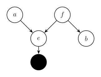
This leads to asking a more general question. Are $a$ and $b$ conditionally independent given $c$ ? (see Figure 4)

Or, in more general, isa given subset of variables $\mathcal{A}$ independent of another set $\mathcal{B}$ conditioned on a third subset $\mathcal{C}$ ? ( $\mathsf{x}_{\mathcal{A}} \perp \mathsf{x}_{\mathcal{B}} \mid \mathsf{x}_{\mathcal{C}}$ ) Thus, the goal is to determine independencies directly from the directed acyclic graph.

We can define the concept of $d$ -separation as. If all paths from any node in $\mathcal{A}$ to any node in $\mathcal{B}$ given the nodes in $\mathcal{C}$ are blocked, then $\mathcal{A} \perp \mathcal{B} \mid \mathcal{C}$ .

Or more formally as.

Let $G$ be a directed graph and $\mathcal{A}$ , $\mathcal{B}$ , and $\mathcal{C}$ disjoint sets of nodes. Then, if all paths from any node in $\mathcal{A}$ to any node in $\mathcal{B}$ given the nodes in $\mathcal{C}$ are blocked, $\mathcal{A}$ and $\mathcal{B}$ are said to be $d$ -separated by $\mathcal{C}$ and $\mathcal{A} \perp \mathcal{B} \mid \mathcal{C}$ .

A path between $\mathcal{A}$ and $\mathcal{B}$ is blocked if the path includes either,

A head-to-tail or tail-to-tail node which is in $\mathcal{C}$ , or,
A head-to-head node, and neither the node nor any of its descendants in $\mathcal{C}$ .

So, to answer our question to Figure 4.

Path from $a$ to $b$ are not blocked by $f$ , since a tail-to-tail node and $f$ is unobserved.

Path not blocked by $e$ , as a head-to-head node with an observed descendant.

Thus, $a \perp b \mid f$ does not hold from the DAG.

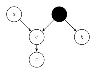
Are $a$ and $b$ conditionally independent given $f$ ?

Path from $a$ to $b$ are blocked by $f$ , since a tail-to-tail node and $f$ is observed. Path blocked by $e$ , as a head-to-head node and neither the node nor any of its descendants are observed.

Hence, $a \perp b \mid f$ holds from the DAG.

Note (Markov Blanket)

In a directed graphical model, a node is conditionally independent of all other nodes given its parents, children and co-parnets.

The Markov blanket of node $\mathsf{x}_i$ is the minimal set of nodes that isolates $\mathsf{x}_i$ from the rest of the graph.

Note (Structured Learning)

What if the Bayesian network is not known? (i.e., we do not know the structure of the graph)

Bayesian networks can be learned from data without a pre-specified structure.

Different algorithms can be employed to learn network structure by analyzing the data and inferring most likely graph structure that best fits observed dependencies.
Once structure and parameters are learned, the Bayesian network can be used for prediction.