Part 8 - Graphical Models III

Introduction

In this part, we will introduce (exact) inference in graphical models, using factor graphs and the sum-product algorithm.

Inference in Graphical Models

Intuition (Inference in Graphical Models)

So far, we have discussed how to represent complex distributions using graphical models (Bayesian networks and MRFs) and how to perform efficient sampling using ancestral sampling. However, another important task is to perform inference, i.e., compute marginal distributions or conditional distributions of certain variables given evidence. This task involves computing posterior probabilities of unobserved variables given observed ones.

Recall (Probabilistic Models)

Discriminative Probabilistic Models: Learn model $p(y \mid \mathbf{x}, \mathbf{w}, \beta)$
Generative Probabilistic Models: Obtain $p(y \mid \mathbf{x}, \mathbf{w}, \beta)$ from learned model $p(\mathbf{x}, y \mid \mathbf{w}, \beta)$ .
Bayesian Supervised Learning: Obtain $p(y \mid \mathcal{D}, \mathbf{x}, \beta)$ by evaluating $p(\mathbf{w} \mid \mathcal{D}, \beta)$ .

Can we explort the graph structure to devise efficient algorithms for inference?

Exact Inference on a Chain Graph

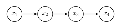
Example 1 (Exact Inference on a Chain Graph)

Consider the chain graph in Figure 1, where we want to compute the marginal distribution $p(x_4)$ .

The direct approach would be, assuming our variables are discrete and can take $K$ possible values,

p(x_4) \coloneqq \sum_{x_1} \sum_{x_2} \sum_{x_3} p(x_1, x_2, x_3, x_4)

However, the complexity is $\mathcal{O}(K^4)$ , or in the general case $\mathcal{O}(K^N)$ for $N$ variables.

But, we know that we can exploit factorization, i.e., $p(x_1, x_2, x_3, x_4) = p(x_1) p(x_2 \mid x_1) p(x_3 \mid x_2) p(x_4 \mid x_3)$ ,

\begin{align*} p(x_4) & = \sum_{x_1} \sum_{x_2} \sum_{x_3} p(x_1) p(x_2 \mid x_1) p(x_3 \mid x_2) p(x_4 \mid x_3) \newline & = \sum_{x_2} \sum_{x_3} \left[ \underbrace{\sum_{x_1} p(x_1) p(x_2 \mid x_1)}_{\mu_2(x_2)} \right] p(x_3 \mid x_2) p(x_4 \mid x_3) \newline & = \sum_{x_3} \left[ \underbrace{\sum_{x_2} \mu_2(x_2) p(x_3 \mid x_2)}_{\mu_3(x_3)} \right] p(x_4 \mid x_3) \newline & = \underbrace{\sum_{x_3} \mu_3(x_3) p(x_4 \mid x_3)}_{\mu_4(x_4)} \end{align*}

Thus,

\begin{align*} p(x_4) & = \sum_{x_1} \sum_{x_2} \sum_{x_3} p(x_1) p(x_2 \mid x_1) p(x_3 \mid x_2) p(x_4 \mid x_3) \newline & = \sum_{x_3} \left[ \sum_{x_2} \left[ \sum_{x_1} p(x_1) p(x_2 \mid x_1) \right] p(x_3 \mid x_2) \right] p(x_4 \mid x_3) \newline \end{align*}

The complexity is now $\mathcal{O}(3K^2)$ , or in the general case $\mathcal{O}(NK^2)$ for $N$ variables.

Note (Message Passing)

The intermediate quantities $\mu_2(x_2), \mu_3(x_3), \mu_4(x_4)$ are called messages, and the procedure of computing marginal distributions by passing messages along the graph is called message passing. $mu_2(x_2)$ is the message from $x_2$ to $x_3$ , $mu_3(x_3)$ is the message from $x_3$ to $x_4$ , obtained by multiplying $\mu_2(x_2)$ with a local function and similarly for $\mu_4(x_4)$ .

Thus, marginalization can be performed by message passing along the chain graph.

Factor Graphs and the Sum-Product Algorithm

Intuition (Message Passing)

The idea of message passing on a chain can be generalized to more general graphical models.

In directed and undirected graphs, it allows us to express global functions as a product of factors over a subset of the variables.

So called, factor graphs, they make decompositions explicitly by introducing additional factor nodes.

Definition 1 (Factor Graph)

Introduced by Frey, Kschischang, Loeliger and Wiberg (1997) [^1], they are a powerful graphical model to reprsent explicitly the factorization of a joint distribution as a product of local factors.

They naturally lead to a message passing algorithm (sum-product algorithm, belief propagation) for efficient in4

They consist of a collection of variables $\mathbf{x} = (x_1, \ldots, x_n), x_i \in \mathcal{A}_i$ and a set of factors (functions) $g(x_1, \ldots, x_n)$ ,

g : \mathcal{A}_1 \times \ldots \times \mathcal{A}_n \to \mathbb{R}

Assume that $g(\mathbf{x})$ can be factorized as,

g(\mathbf{x}) = \prod_{j \in \mathcal{J}} f_j(\mathcal{X}_j)

where we call $g(\cdot)$ the global function, $f_j(\cdot)$ the local functions, $\mathcal{J}$ is the discrete index set and $\mathcal{X}_j$ is a subset of variables in $\mathbf{x}$ .

More formally we say that, a bipartite graph that expresses the structure of the factorization,

g(\mathbf{x}) = \prod_{j \in \mathcal{J}} f_j(\mathcal{X}_j)

The factor graph has one variable node for each variable $x_i$ , one factor node for each local function $f_j$ , and an undirected edge connecting a variable node $x_i$ with a factor node $f_j$ if and only if $x_i$ is an argument of $f_j$ .

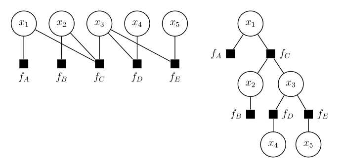
Example 2 (Factor Graph Example)

Consider the factor graph in Figure 2, representing the factorization, the corresponding global function is,

g(x_1, x_2, x_3, x_4, x_5) \coloneqq f_A(x_1) f_B(x_2) f_C(x_1, x_2, x_3) f_D(x_3, x_4) f_E(x_3, x_5)

To go from a directed graph to a factor graph we,

Add one factor for each node
Connect variable nodes to factor nodes according to edges

In the undirected case, we instead,

Add one factor for each maximal clique
Connect variable nodes to clique factors.

Intuition (Marginal Functions)

Factor graphs are a tool for efficient computation of marginal functions when $g(\mathbf{x})$ represents a probability distribution and the corresponding factor graph is cycle-free (i.e., exact marginalization).

Marginalization can be computed by message passing over the factor graph, for example, the marginal with respect to $x_i$ ,

\begin{align*} g_i(x_i) & \coloneqq \sum_{x_1} \ldots \sum_{x_{i-1}} \sum_{x_{i+1}} \ldots \sum_{x_n} g(x_1, \ldots, x_n) \newline & = \sum_{\sim x_i} g(x_1, \ldots, x_n) \newline \end{align*}

Thus, we can perform marginalization via message passing over the factor graph by exploiting the factorization and the distributive law and reusing partials sums.

Note (Distributive Law)

Let $\mathcal{F}$ be a set of elements on which two binary operations, “ $+$ ” and “ $\cdot$ ”, are defined. The operation “ $\cdot$ ” is said to be distributive over “ $+$ ” if for all $a, b, c \in \mathcal{F}$ ,

a \cdot (b + c) = a \cdot b + a \cdot c

and,

(b + c) \cdot a = b \cdot a + c \cdot

Intuition (Message Passing (Continued))

A (general) message passing algorithm to compute marginalization involves,

Computation of marginal begins at the leaves of the tree.
Has the following operations:
- Variable node: Product of incoming messages from children; Forwards result to parent.
- Factor node: Product of incoming messages and local function $f_j(\mathcal{X}_j)$ , applies to it not-sum operator; Forwards result to parent.
Marginalization terminates at root node $g_i(x_i)$ obtained as product of all incoming messages to root node $x_i$ .
Notation:
- $\mu_{x \to f}$ : message from VN $x$ to FN $f$ .
- $\mu_{f \to x}$ : message from FN $f$ to VN $x$ .
Operations (with notation):
- Leaf VN: $\mu_{x \to f} = 1$ .
- Single-Child VN: forwards incoming message.
- Leaf FN $\mu_{f_B \to x_2} = \sum_{\sim x_2} f_B(x_2) = f_B(x_2)$ (See Figure 2).
- Single-Child FN: $\mu_{f_E \to x_3} = \sum_{\sim x_3} f_E(x_3, x_5)$ (See Figure 2).

Algorithm (Sum-Product Algorithm)

But how do we compute several (or all) marginals $g_i(x_i)$ ?

If we perfor message passing separately for each marginal $g_i(x_i)$ , we would be repeating many calculations and thus wastefully increasing computational complexity. If we can perform message passing simultaneously and compute the marginals for all variables at once, we can reuse many intermediate results.

The algorithm initiates at the leave sof the tree, the leaf VN $x$ sends $\mu_{x \to f} = 1$ ; leaf FN $f$ sends $\mu_{f \to x} = f(x)$ . A message from a node to one of its neighbors is computed once all messages from all other neighbors are received.

The variable node update can be defined as,

\mu_{x \to f} \coloneqq \prod_{f^{\prime} \in \mathcal{N}(x) \backslash f} \mu_{f^{\prime} \to x}

and the factor node update as,

\mu_{f \to x} \coloneqq \sum_{\sim x} \left(f(\mathcal{X}) \prod_{x^{\prime} \in \mathcal{N}(f) \backslash x} \mu_{x^{\prime} \to f}\right)

The algorithm terminates once two messages have been passed over ever edge.

$g_i(x_i)$ is obtained as the product of all incoming messages to VN $x_i$ .

Intuition (The sum-product Algorithm with Observed Variables)

In most applications, some variables are observed, and we want to compute the posterior conditioned on some observed variables. For each observed variable, we add a Dirac delta/indicator factor. Thus, the factor graph describes,

\begin{align*} p(\mathbf{x}) \prod_{x \in \mathcal{X}} \delta(x - x_{\text{obs}}) \newline & = p(\mathbf{x} \backslash \mathcal{X}, \mathcal{X} = \mathcal{X}_{\text{obs}}) \propto p(\mathbf{x} \backslash \mathcal{X} \mid \mathcal{X} = \mathcal{X}_{\text{obs}}) \end{align*}

where $\mathcal{X}$ is the set of all observed variables.

The posterior marginals $p(x_i \mid \mathcal{X} = \mathcal{X}_{\text{obs}})$ can be computed by the sum-product algorithm $(x_i \in \mathcal{A})$ where $\mathcal{A}$ is the set of unobserved variables.

Bayes’ Theorem through a Message Passing Lens

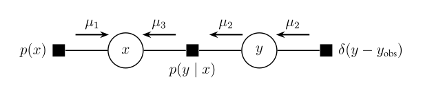
Example 3 (Bayes’ Theorem through a Message Passing Lens)

Consider the graphical model in Figure 3.

Our latent variable is $x$ and our observed variable is $y = y_{\text{obs}}$ and our objective is to infer $p(x \mid y)$ .

We know from Bayes’ theorem that,

p(x \mid y) = \frac{p(y \mid x) p(x)}{p(y)} \propto p(y \mid x) p(x)

Note that $p(x, y) = p(y \mid x) p(x)$ . Thus,

p(x \mid y_{\text{obs}}) \propto \mu_1(x) \mu_3(x) = p(x) p(y_{\text{obs}} \mid x)

where $\mu_1(x) = p(x)$ , $\mu_2(x) = \delta(y - y_{\text{obs}})$ , and $\mu_3(x) = \int p(y \mid x) \mu_2(y) \ dy = p(y_{\text{obs}} \mid x)$ (See Figure 3).

Note (The Sum-Product Algorithm in Factor Graphs with Cycles)

One of the limitations of the sum-product algorithm is that it only provides exact marginals for cycle-free factor graphs.

If our factor graphs contains cycles, then no natural termination of the algorithm exists, instead we can use it as an iterative algorithm, it might strictly be suboptiomal, but it still gives excellent results in many cases!

One final note, if the objective is to find a configuration of the variables with the largest probability, this can be performed via the max-sum algorithm,

\mathbf{x}_{\text{max}} = \underset{\mathbf{x}}{\arg\max} \ p(\mathbf{x})