Introduction
We have previously discussed Abadie’s constraint qualifications and the Karush-Kuhn-Tucker (KKT) conditions.
However, Abadie’s constraint qualifications does not hold always (of course :)).
Further, checking Abadie’s constraint qualifications requires us to compute the tangent cone T S ( x ∗ ) T_S(\mathbf{x}^*) T S ( x ∗ )
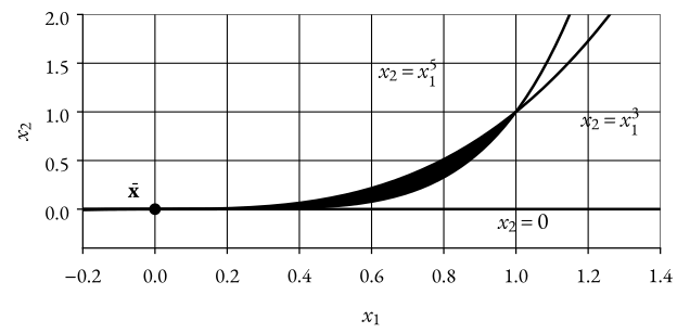
Example 1 Let,
S = { g 1 ( x ) = − x 1 3 + x 2 ≤ 0 g 2 ( x ) = x 1 5 − x 2 ≤ 0 g 3 ( x ) = − x 2 ≤ 0 S = \begin{cases}
g_1(\mathbf{x}) = -x_1^3 + x_2 \leq 0 \newline
g_2(\mathbf{x}) = x_1^5 - x_2 \leq 0 \newline
g_3(\mathbf{x}) = -x_2 \leq 0
\end{cases} S = ⎩ ⎨ ⎧ g 1 ( x ) = − x 1 3 + x 2 ≤ 0 g 2 ( x ) = x 1 5 − x 2 ≤ 0 g 3 ( x ) = − x 2 ≤ 0 Further, let x ˉ = ( 0 0 ) T \bar{\mathbf{x}} = \begin{pmatrix} 0 & 0 \end{pmatrix}^T x ˉ = ( 0 0 ) T T S ( x ˉ ) T_S(\bar{\mathbf{x}}) T S ( x ˉ ) G ( x ˉ ) G(\bar{\mathbf{x}}) G ( x ˉ )
Figure 1: Feasible region and constraintsLet x 1 k = 1 k x_1^k = \frac{1}{k} x 1 k = k 1 g 1 ( x ) g_1(\mathbf{x}) g 1 ( x ) x 2 k ≤ 1 k 3 x_2^k \leq \frac{1}{k^3} x 2 k ≤ k 3 1
Further, let x 2 k x_2^k x 2 k ≥ 0 , ∀ k \geq 0, \forall k ≥ 0 , ∀ k g 3 ( x ) g_3(\mathbf{x}) g 3 ( x )
Then,
lim k → ∞ x k = x ˉ λ k ( x k − x ˉ ) = [ λ k k λ k x 2 k ] \begin{align*}
\lim_{k \to \infty} x^k = \bar{\mathbf{x}} \newline
\lambda^k (\mathbf{x}^k - \bar{\mathbf{x}}) = \begin{bmatrix}
\frac{\lambda^k}{k} \newline
\lambda^k x_2^k
\end{bmatrix}
\end{align*} k → ∞ lim x k = x ˉ λ k ( x k − x ˉ ) = [ k λ k λ k x 2 k ] Thus, we must select a λ k \lambda^k λ k λ k k → \frac{\lambda^k}{k} \to k λ k → > 0 > 0 > 0 k → ∞ k \to \infty k → ∞
But then, 0 ≤ λ k x 2 k ≤ λ k k 3 → 0 0 \leq \lambda^k x_2^k \leq \frac{\lambda^k}{k^3} \to 0 0 ≤ λ k x 2 k ≤ k 3 λ k → 0 k → ∞ k \to \infty k → ∞
So, T S ( x ˉ ) = { p ∈ R 2 ∣ p 1 ≥ 0 , p 2 = 0 } T_S(\bar{\mathbf{x}}) = \{\mathbf{p} \in \mathbb{R}^2 \mid p_1 \geq 0, p_2 = 0\} T S ( x ˉ ) = { p ∈ R 2 ∣ p 1 ≥ 0 , p 2 = 0 }
For the gradient cone,
{ ∇ g 1 ( x ) = [ − 3 x 1 2 1 ] T ⟹ ∇ g 1 ( x ˉ ) = [ 0 1 ] T ∇ g 2 ( x ) = [ 5 x 1 4 − 1 ] T ⟹ ∇ g 2 ( x ˉ ) = [ 0 − 1 ] T ∇ g 3 ( x ) = [ 0 − 1 ] T ⟹ ∇ g 3 ( x ˉ ) = [ 0 − 1 ] T ⟹ { ∇ g 1 ( x ˉ ) T p = 0 ⋅ p 1 + 1 ⋅ p 2 = p 2 ≤ 0 ∇ g 2 ( x ˉ ) T p = 0 ⋅ p 1 − 1 ⋅ p 2 = − p 2 ≤ 0 ∇ g 3 ( x ˉ ) T p = 0 ⋅ p 1 − 1 ⋅ p 2 = − p 2 ≤ 0 ⟹ G ( x ˉ ) = { p ∈ R 2 ∣ p 2 ≤ 0 , − p 2 ≤ 0 } = { p ∈ R 2 ∣ p 2 = 0 } \begin{align*}
&
\begin{cases}
\nabla g_1(\mathbf{x}) = \begin{bmatrix} -3x_1^2 & 1 \end{bmatrix}^T \implies \nabla g_1(\bar{\mathbf{x}}) = \begin{bmatrix} 0 & 1 \end{bmatrix}^T \newline
\nabla g_2(\mathbf{x}) = \begin{bmatrix} 5x_1^4 & -1 \end{bmatrix}^T \implies \nabla g_2(\bar{\mathbf{x}}) = \begin{bmatrix} 0 & -1 \end{bmatrix}^T \newline
\nabla g_3(\mathbf{x}) = \begin{bmatrix} 0 & -1 \end{bmatrix}^T \implies \nabla g_3(\bar{\mathbf{x}}) = \begin{bmatrix} 0 & -1 \end{bmatrix}^T
\end{cases}
\implies \newline
&
\begin{cases}
\nabla g_1(\bar{\mathbf{x}})^T \mathbf{p} = 0 \cdot p_1 + 1 \cdot p_2 = p_2 \leq 0 \newline
\nabla g_2(\bar{\mathbf{x}})^T \mathbf{p} = 0 \cdot p_1 - 1 \cdot p_2 = -p_2 \leq 0 \newline
\nabla g_3(\bar{\mathbf{x}})^T \mathbf{p} = 0 \cdot p_1 - 1 \cdot p_2 = -p_2 \leq 0
\end{cases}
\implies \newline
&
G(\bar{\mathbf{x}}) = \{\mathbf{p} \in \mathbb{R}^2 \mid p_2 \leq 0, -p_2 \leq 0\} = \{\mathbf{p} \in \mathbb{R}^2 \mid p_2 = 0\}
\end{align*} ⎩ ⎨ ⎧ ∇ g 1 ( x ) = [ − 3 x 1 2 1 ] T ⟹ ∇ g 1 ( x ˉ ) = [ 0 1 ] T ∇ g 2 ( x ) = [ 5 x 1 4 − 1 ] T ⟹ ∇ g 2 ( x ˉ ) = [ 0 − 1 ] T ∇ g 3 ( x ) = [ 0 − 1 ] T ⟹ ∇ g 3 ( x ˉ ) = [ 0 − 1 ] T ⟹ ⎩ ⎨ ⎧ ∇ g 1 ( x ˉ ) T p = 0 ⋅ p 1 + 1 ⋅ p 2 = p 2 ≤ 0 ∇ g 2 ( x ˉ ) T p = 0 ⋅ p 1 − 1 ⋅ p 2 = − p 2 ≤ 0 ∇ g 3 ( x ˉ ) T p = 0 ⋅ p 1 − 1 ⋅ p 2 = − p 2 ≤ 0 ⟹ G ( x ˉ ) = { p ∈ R 2 ∣ p 2 ≤ 0 , − p 2 ≤ 0 } = { p ∈ R 2 ∣ p 2 = 0 } We can see that T S ( x ˉ ) ⊆ G ( x ˉ ) T_S(\bar{\mathbf{x}}) \subseteq G(\bar{\mathbf{x}}) T S ( x ˉ ) ⊆ G ( x ˉ ) T S ( x ˉ ) ≠ G ( x ˉ ) T_S(\bar{\mathbf{x}}) \neq G(\bar{\mathbf{x}}) T S ( x ˉ ) = G ( x ˉ )
Constraint Qualifications
We will now introduce some more constraint qualifications that are easier to check than Abadie’s constraint qualifications, but imply that Abadie’s constraint qualifications hold.
Definition 1 (Linear Independence Constraint Qualification (LICQ)) The Linear Independence Constraint Qualification (LICQ) holds at a point x ⋆ \mathbf{x}^{\star} x ⋆ ∇ g i ( x ⋆ ) , i ∈ I ( x ⋆ ) \nabla g_i(\mathbf{x}^{\star}), i \in \mathcal{I}(\mathbf{x}^{\star}) ∇ g i ( x ⋆ ) , i ∈ I ( x ⋆ )
Theorem 1 LICQ ⟹ Abadie’s CQ \text{LICQ} \implies \text{Abadie's CQ} LICQ ⟹ Abadie’s CQ Definition 2 (Affine Independence Constraint Qualification (Affine CQ)) The Affine Independence Constraint Qualification (Affine CQ) holds if all g i ( x ) , i ∈ I ( x ⋆ ) g_i(\mathbf{x}), i \in \mathcal{I}(\mathbf{x}^{\star}) g i ( x ) , i ∈ I ( x ⋆ ) ∇ g i ( x ⋆ ) , i = 1 , … , m \nabla g_i(\mathbf{x}^{\star}), i = 1, \ldots, m ∇ g i ( x ⋆ ) , i = 1 , … , m
Theorem 2 Affine CQ ⟹ Abadie’s CQ. (In all points x ∈ S ) \text{Affine CQ} \implies \text{Abadie's CQ. (In all points } \mathbf{x} \in S\text{)} Affine CQ ⟹ Abadie’s CQ. (In all points x ∈ S ) Definition 3 (Slater’s Constraint Qualification (Slater’s CQ)) Slater’s Constraint Qualification (Slater’s CQ) holds if all g i ( x ) , i = 1 , … , m g_i(\mathbf{x}), i = 1, \ldots, m g i ( x ) , i = 1 , … , m ∃ x 0 such that g i ( x 0 ) < 0 , i = 1 , … , m \exists\, \mathbf{x}_0 \, \text{such that} \quad g_i(\mathbf{x}_0) < 0, i = 1, \ldots, m ∃ x 0 such that g i ( x 0 ) < 0 , i = 1 , … , m
Theorem 3 Slater’s CQ ⟹ Abadie’s CQ. (In all points x ∈ S ) \text{Slater's CQ} \implies \text{Abadie's CQ. (In all points } \mathbf{x} \in S\text{)} Slater’s CQ ⟹ Abadie’s CQ. (In all points x ∈ S ) Karush-Kuhn-Tucker (KKT) Conditions with Equality Constraints
So far, we have only considered inequality constraints when discussing the KKT conditions.
Let’s see how we can extend the KKT conditions to also include equality constraints.
Consider the following optimization problem with both equality and inequality constraints,
min f ( x ) subject to g i ( x ) ≤ 0 , i = 1 , … , m h j ( x ) = 0 , j = 1 , … , l \begin{align*}
\min & f(\mathbf{x}) \newline
\text{subject to} \quad & g_i(\mathbf{x}) \leq 0, i = 1, \ldots, m \newline
\ & h_j(\mathbf{x}) = 0, j = 1, \ldots, l
\end{align*} min subject to f ( x ) g i ( x ) ≤ 0 , i = 1 , … , m h j ( x ) = 0 , j = 1 , … , l Let’s do a trick and reformulate the problem as,
min f ( x ) subject to g i ( x ) ≤ 0 , i = 1 , … , m h j ( x ) ≤ 0 , j = 1 , … , l − h j ( x ) ≤ 0 , j = 1 , … , l \begin{align*}
\min & f(\mathbf{x}) \newline
\text{subject to} \quad & g_i(\mathbf{x}) \leq 0, i = 1, \ldots, m \newline
\ & h_j(\mathbf{x}) \leq 0, j = 1, \ldots, l \newline
\ & -h_j(\mathbf{x}) \leq 0, j = 1, \ldots, l
\end{align*} min subject to f ( x ) g i ( x ) ≤ 0 , i = 1 , … , m h j ( x ) ≤ 0 , j = 1 , … , l − h j ( x ) ≤ 0 , j = 1 , … , l Thus, the KKT conditions for this problem are,
{ ∇ f ( x ⋆ ) + ∑ i = 1 m μ i ∇ g i ( x ⋆ ) + ∑ j = 1 l λ 1 , j ∇ h j ( x ⋆ ) + ∑ j = 1 l λ 2 , j ∇ ( − h j ( x ⋆ ) ) ⏟ = ∑ j = 1 l ( λ 1 , j − λ 2 , j ) ∇ h j ( x ⋆ ) = 0 μ i g i ( x ⋆ ) = 0 , i = 1 , … , m Always fulfilled for feasible x ⋆ , { λ 1 , j h j ( x ⋆ ) = 0 , j = 1 , … , l λ 2 , j ( − h j ( x ⋆ ) ) = 0 , j = 1 , … , l μ i , λ 1 , j , λ 2 , j ≥ 0 , i = 1 , … , m , j = 1 , … , l \begin{cases}
\nabla f(\mathbf{x}^{\star}) + \sum_{i=1}^{m} \mu_i \nabla g_i(\mathbf{x}^{\star}) + \underbrace{\sum_{j=1}^{l} \lambda_{1, j} \nabla h_j(\mathbf{x}^{\star}) + \sum_{j=1}^{l} \lambda_{2, j} \nabla (-h_j(\mathbf{x}^{\star}))}_{= \sum_{j=1}^{l} (\lambda_{1, j} - \lambda_{2, j}) \nabla h_j(\mathbf{x}^{\star})} = 0 \newline
\mu_i g_i(\mathbf{x}^{\star}) = 0, i = 1, \ldots, m \newline
\text{Always fulfilled for feasible } \mathbf{x}^{\star},
\begin{cases}
\lambda_{1, j} h_j(\mathbf{x}^{\star}) = 0, j = 1, \ldots, l \newline
\lambda_{2, j} (-h_j(\mathbf{x}^{\star})) = 0, j = 1, \ldots, l \newline
\end{cases} \newline
\mu_i, \lambda_{1, j}, \lambda_{2, j} \geq 0, i = 1, \ldots, m, j = 1, \ldots, l \newline
\end{cases} ⎩ ⎨ ⎧ ∇ f ( x ⋆ ) + ∑ i = 1 m μ i ∇ g i ( x ⋆ ) + = ∑ j = 1 l ( λ 1 , j − λ 2 , j ) ∇ h j ( x ⋆ ) j = 1 ∑ l λ 1 , j ∇ h j ( x ⋆ ) + j = 1 ∑ l λ 2 , j ∇ ( − h j ( x ⋆ )) = 0 μ i g i ( x ⋆ ) = 0 , i = 1 , … , m Always fulfilled for feasible x ⋆ , { λ 1 , j h j ( x ⋆ ) = 0 , j = 1 , … , l λ 2 , j ( − h j ( x ⋆ )) = 0 , j = 1 , … , l μ i , λ 1 , j , λ 2 , j ≥ 0 , i = 1 , … , m , j = 1 , … , l Thus, let λ j = λ 1 , j − λ 2 , j \lambda_j = \lambda_{1, j} - \lambda_{2, j} λ j = λ 1 , j − λ 2 , j λ j ∈ R \lambda_j \in \mathbb{R} λ j ∈ R
{ ∇ f ( x ⋆ ) + ∑ i = 1 m μ i ∇ g i ( x ⋆ ) + ∑ j = 1 l λ j ∇ h j ( x ⋆ ) = 0 μ i g i ( x ⋆ ) = 0 , i = 1 , … , m μ i ≥ 0 , i = 1 , … , m (*) \begin{cases}
\nabla f(\mathbf{x}^{\star}) + \sum_{i=1}^{m} \mu_i \nabla g_i(\mathbf{x}^{\star}) + \sum_{j=1}^{l} \lambda_j \nabla h_j(\mathbf{x}^{\star}) = 0 \newline
\mu_i g_i(\mathbf{x}^{\star}) = 0, i = 1, \ldots, m \newline
\mu_i \geq 0, i = 1, \ldots, m \newline
\end{cases}
\tag{*} ⎩ ⎨ ⎧ ∇ f ( x ⋆ ) + ∑ i = 1 m μ i ∇ g i ( x ⋆ ) + ∑ j = 1 l λ j ∇ h j ( x ⋆ ) = 0 μ i g i ( x ⋆ ) = 0 , i = 1 , … , m μ i ≥ 0 , i = 1 , … , m ( * ) Now to fully generalize and capture the KKT conditions with equality constraints, we need to define a new cone.
Definition 4 (Tangent Space Cone for Equality Constraints) H ( x ) ≔ { p ∈ R n ∣ ∇ h j ( x ) T p = 0 , j = 1 , … , l } H(\mathbf{x}) \coloneqq \{\mathbf{p} \in \mathbb{R}^n \mid \nabla h_j(\mathbf{x})^T \mathbf{p} = 0, j = 1, \ldots, l\} H ( x ) : = { p ∈ R n ∣ ∇ h j ( x ) T p = 0 , j = 1 , … , l } With this we can define Abadie’s constraint qualifications for problems with equality constraints.
Definition 5 (Abadie’s Constraint Qualifications with Equality Constraints) Abadie’s constraint qualifications hold at a point x ⋆ ∈ S \mathbf{x}^{\star} \in S x ⋆ ∈ S
T S ( x ⋆ ) = G ( x ⋆ ) ∩ H ( x ⋆ ) T_S(\mathbf{x}^{\star}) = G(\mathbf{x}^{\star}) \cap H(\mathbf{x}^{\star}) T S ( x ⋆ ) = G ( x ⋆ ) ∩ H ( x ⋆ ) Theorem 4 (KKT Conditions with Equality Constraints) Assume Abadie’s constraint qualifications hold in x ⋆ ∈ S \mathbf{x}^{\star} \in S x ⋆ ∈ S
x ⋆ is a local minimum ⟹ The system (*) is solvable for μ and λ . \mathbf{x}^{\star} \text{ is a local minimum } \implies \text{The system (*) is solvable for } \boldsymbol{\mu} \text{ and } \boldsymbol{\lambda}. x ⋆ is a local minimum ⟹ The system (*) is solvable for μ and λ . We can now define the sufficient conditions for optimality with equality constraints.
Theorem 5 (Sufficient Conditions for Optimality with Equality Constraints) Assume that f ( x ) f(\mathbf{x}) f ( x ) S S S ∀ g i ( x ) , i = 1 , … , m \forall g_i(\mathbf{x}), i = 1, \ldots, m ∀ g i ( x ) , i = 1 , … , m S S S ∀ h j ( x ) , j = 1 , … , l \forall h_j(\mathbf{x}), j = 1, \ldots, l ∀ h j ( x ) , j = 1 , … , l S S S
x ⋆ is a KKT point ⟹ x ⋆ is globally optimal. \mathbf{x}^{\star} \text{ is a KKT point } \implies \mathbf{x}^{\star} \text{ is globally optimal.} x ⋆ is a KKT point ⟹ x ⋆ is globally optimal. Proof (Sufficient Conditions for Optimality with Equality Constraints) Let x ⋆ \mathbf{x}^{\star} x ⋆ g i ( x ) , ∀ x ∈ S g_i(\mathbf{x}), \forall \mathbf{x} \in S g i ( x ) , ∀ x ∈ S i ∈ I ( x ⋆ ) i \in \mathcal{I}(\mathbf{x}^{\star}) i ∈ I ( x ⋆ ) C 1 C^1 C 1
∇ g i ( x ⋆ ) T ( x − x ⋆ ) ≤ g i ( x ) ⏟ ≤ 0 − g i ( x ⋆ ) ⏟ = 0 since i ∈ I ( x ⋆ ) ≤ 0 \begin{align*}
\nabla g_i(\mathbf{x}^{\star})^T (\mathbf{x} - \mathbf{x}^{\star}) & \leq \underbrace{g_i(\mathbf{x})}_{\leq 0} - \underbrace{g_i(\mathbf{x}^{\star})}_{= \ 0 \text{ since } i \in \mathcal{I}(\mathbf{x}^{\star})} \newline
& \leq 0
\end{align*} ∇ g i ( x ⋆ ) T ( x − x ⋆ ) ≤ ≤ 0 g i ( x ) − = 0 since i ∈ I ( x ⋆ ) g i ( x ⋆ ) ≤ 0 Since h j ( x ) , j = 1 , … , l h_j(\mathbf{x}), j = 1, \ldots, l h j ( x ) , j = 1 , … , l C 1 C^1 C 1 1
∇ h j ( x ⋆ ) T ( x − x ⋆ ) = h j ( x ) ⏟ = 0 − h j ( x ⋆ ) ⏟ = 0 = 0 \begin{align*}
\nabla h_j(\mathbf{x}^{\star})^T (\mathbf{x} - \mathbf{x}^{\star}) & = \underbrace{h_j(\mathbf{x})}_{= \ 0} - \underbrace{h_j(\mathbf{x}^{\star})}_{= \ 0} \newline
& = 0
\end{align*} ∇ h j ( x ⋆ ) T ( x − x ⋆ ) = = 0 h j ( x ) − = 0 h j ( x ⋆ ) = 0 Further, by convexity of f ( x ) f(\mathbf{x}) f ( x ) ∀ x ∈ S \forall \mathbf{x} \in S ∀ x ∈ S
f ( x ) − f ( x ⋆ ) ≥ ∇ f ( x ⋆ ) T ( x − x ⋆ ) ≥ ( − ∑ i = 1 m μ i ⏟ ≥ 0 ∇ g i ( x ⋆ ) ⏟ ≤ 0 ⏟ ≤ 0 ⏟ ≤ 0 ⏟ ≥ 0 − ∑ j = 1 l λ j ∇ h j ( x ⋆ ) ⏟ = 0 ) T ( x − x ⋆ ) ≥ 0 \begin{align*}
f(\mathbf{x}) - f(\mathbf{x}^{\star}) & \geq \nabla f(\mathbf{x}^{\star})^T (\mathbf{x} - \mathbf{x}^{\star}) \newline
& \geq \left(\underbrace{- \underbrace{\sum_{i=1}^{m} \underbrace{\underbrace{\mu_i}_{\geq 0} \underbrace{\nabla g_i(\mathbf{x}^{\star})}_{\leq 0}}_{\leq 0}}_{\leq 0}}_{\geq 0} - \underbrace{\sum_{j=1}^{l} \lambda_j \nabla h_j(\mathbf{x}^{\star})}_{= \ 0}\right)^T (\mathbf{x} - \mathbf{x}^{\star}) \newline
& \geq 0
\end{align*} f ( x ) − f ( x ⋆ ) ≥ ∇ f ( x ⋆ ) T ( x − x ⋆ ) ≥ ≥ 0 − ≤ 0 i = 1 ∑ m ≤ 0 ≥ 0 μ i ≤ 0 ∇ g i ( x ⋆ ) − = 0 j = 1 ∑ l λ j ∇ h j ( x ⋆ ) T ( x − x ⋆ ) ≥ 0 Thus, by definition of global optimality, x ⋆ \mathbf{x}^{\star} x ⋆
Connection to Lagrangian Relaxation
We can also connect the KKT conditions to the Lagrangian relaxation.
Let’s first define the Lagrangian.
Definition 6 (Lagrangian) For the problem,
min f ( x ) subject to g i ( x ) ≤ 0 , i = 1 , … , m \begin{align*}
\min & f(\mathbf{x}) \newline
\text{subject to} \quad & g_i(\mathbf{x}) \leq 0, i = 1, \ldots, m \newline
\end{align*} min subject to f ( x ) g i ( x ) ≤ 0 , i = 1 , … , m The Lagrangian is defined as,
L ( x , μ ) = f ( x ) + ∑ i = 1 m μ i g i ( x ) \mathcal{L}(\mathbf{x}, \boldsymbol{\mu}) = f(\mathbf{x}) + \sum_{i=1}^{m} \mu_i g_i(\mathbf{x}) L ( x , μ ) = f ( x ) + i = 1 ∑ m μ i g i ( x ) Note It is not hard to see that,
∇ x L ( x , μ ) = ∇ f ( x ) + ∑ i = 1 m μ i ∇ g i ( x ) ⟹ The first KKT condition is ∇ x L ( x ⋆ , μ ) = 0 \begin{align*}
\nabla_{\mathbf{x}} \mathcal{L}(\mathbf{x}, \boldsymbol{\mu}) & = \nabla f(\mathbf{x}) + \sum_{i=1}^{m} \mu_i \nabla g_i(\mathbf{x}) \newline
& \implies \text{The first KKT condition is } \nabla_{\mathbf{x}} \mathcal{L}(\mathbf{x}^{\star}, \boldsymbol{\mu}) = 0
\end{align*} ∇ x L ( x , μ ) = ∇ f ( x ) + i = 1 ∑ m μ i ∇ g i ( x ) ⟹ The first KKT condition is ∇ x L ( x ⋆ , μ ) = 0 We will now define what relaxtions means.
Definition 7 (Relaxation) For a problem,
( P ) { min f ( x ) subject to x ∈ S \begin{align*}
(P) \quad &
\begin{cases}
\min & f(\mathbf{x}) \newline
\text{subject to} \quad & \mathbf{x} \in S
\end{cases}
\end{align*} ( P ) { min subject to f ( x ) x ∈ S The problem,
( P ′ ) { min f R ( x ) subject to x ∈ S R \begin{align*}
(P^{\prime}) \quad &
\begin{cases}
\min & f_R(\mathbf{x}) \newline
\text{subject to} \quad & \mathbf{x} \in S_R
\end{cases}
\end{align*} ( P ′ ) { min subject to f R ( x ) x ∈ S R The problem ( P ′ ) (P^{\prime}) ( P ′ )
f R ( x ) ≤ f ( x ) , ∀ x ∈ S f_R(\mathbf{x}) \leq f(\mathbf{x}), \forall \mathbf{x} \in S f R ( x ) ≤ f ( x ) , ∀ x ∈ S
S ⊆ S R S \subseteq S_R S ⊆ S R
Lemma 1 (Relaxation Lemma) For μ ≥ 0 \boldsymbol{\mu} \geq \mathbf{0} μ ≥ 0
min L ( x , μ ) subject to x ∈ R n \begin{align*}
\min & \mathcal{L}(\mathbf{x}, \boldsymbol{\mu}) \newline
\text{subject to} \quad & \mathbf{x} \in \mathbb{R^n}
\end{align*} min subject to L ( x , μ ) x ∈ R n is a relaxation of the problem,
min f ( x ) subject to g i ( x ) ≤ 0 , i = 1 , … , m \begin{align*}
\min & f(\mathbf{x}) \newline
\text{subject to} \quad & g_i(\mathbf{x}) \leq 0, i = 1, \ldots, m \newline
\end{align*} min subject to f ( x ) g i ( x ) ≤ 0 , i = 1 , … , m Proof (Relaxation Lemma) By definition, the set S S S R n \mathbb{R}^n R n
S ≔ { x ∈ R n ∣ g i ( x ) ≤ 0 , i = 1 , … , m } ⊆ R n S \coloneqq \{\mathbf{x} \in \mathbb{R}^n \mid g_i(\mathbf{x}) \leq 0, i = 1, \ldots, m\} \subseteq \mathbb{R}^n S : = { x ∈ R n ∣ g i ( x ) ≤ 0 , i = 1 , … , m } ⊆ R n Further, for μ ≥ 0 \boldsymbol{\mu} \geq \mathbf{0} μ ≥ 0 x ∈ S \mathbf{x} \in S x ∈ S
L ( x , μ ) = f ( x ) + ∑ i = 1 m μ i ⏟ ≥ 0 g i ( x ) ⏟ ≤ 0 ⏟ ≤ 0 ≤ f ( x ) \begin{align*}
\mathcal{L}(\mathbf{x}, \boldsymbol{\mu}) & = f(\mathbf{x}) + \underbrace{\sum_{i=1}^{m} \underbrace{\mu_i}_{\geq 0} \underbrace{g_i(\mathbf{x})}_{\leq 0}}_{\leq 0} \newline
& \leq f(\mathbf{x})
\end{align*} L ( x , μ ) = f ( x ) + ≤ 0 i = 1 ∑ m ≥ 0 μ i ≤ 0 g i ( x ) ≤ f ( x ) Theorem 6 (Relaxtion Theorem) a) Let f R ⋆ f_R^{\star} f R ⋆ ( P ′ ) (P^{\prime}) ( P ′ ) f ⋆ f^{\star} f ⋆ ( P ) (P) ( P )
f R ⋆ ≤ f ⋆ f_R^{\star} \leq f^{\star} f R ⋆ ≤ f ⋆ also called the lower bound property.
b) If ( P ′ ) (P^{\prime}) ( P ′ ) ( P ) (P) ( P )
c) If ( P ′ ) (P^{\prime}) ( P ′ ) x R ⋆ ∈ S \mathbf{x}_R^{\star} \in S x R ⋆ ∈ S f R ( x R ⋆ ) = f ( x R ⋆ ) f_R(\mathbf{x}_R^{\star}) = f(\mathbf{x}_R^{\star}) f R ( x R ⋆ ) = f ( x R ⋆ ) x R ⋆ \mathbf{x}_R^{\star} x R ⋆ ( P ) (P) ( P )