We all have heard (yes, pun intended) of decibels. Let’s properly define what decibels are:
Definition 1 (Decibel)∣H(f)∣dB=20log10(∣H(f)∣)
Amplifier
Is just as the name suggests,
V0(t)=AvVi(t).
Note that, Av, can be of any sign, which means we also have inverting amplifiers!
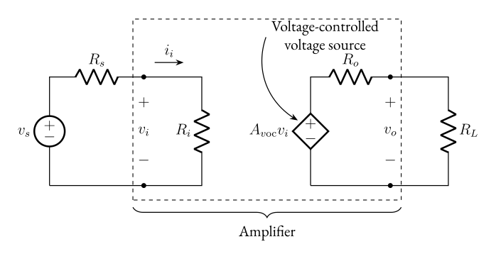
A typical model would look something like:
Figure 2: Model of a voltage amplifier.
Operational Amplifier (Op-Amp)
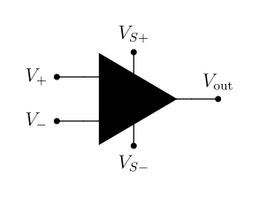
An Op-Amp looks like:
Figure 3: Op-Amp symbol.
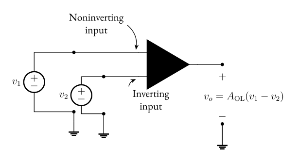
We use the Op-Amp like:
Figure 4: Op-Amp with its inputs.Definition 2 (Ideal Op-Amp)
An Ideal Op-Amp has:
Infinite input impedance
Infinite gain for differential signal
Zero gain for the common-mode signal
Zero output impedance
Infinite bandwidth
Differential signal,
Vd=V1−V2.
Common-mode signal,
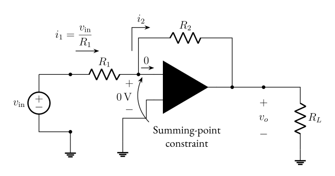
Vcm=21(V1+V2).Figure 5: Inverting amplifier.
Let’s take a look at this Op-Amp circuit,
I1=I2=R1Vin.
KVL,
0+I2R2+VoI2=−R2Vo=0,=R1Vin.
Which means,
Av=VinVo=−R1R2.
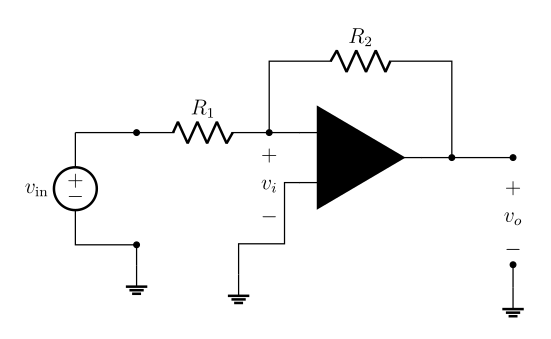
Let’s take a look at this Op-Amp:
Figure 6: Op-Amp with positive feedback.
Here we’ll quickly discover that we have positive feedback. Positive feedback saturates the output - which means we can not use the derived formulas from above!
Always check if there is positive or negative feedback.
For non-inverting amplifiers, we get,
Av=VinVo=1+R1R2.
So, steps to analyze an ideal Op-Amp circuit:
Algorithm 1: Analyzing an ideal Op-Amp circuit
Verify that negative feedback is present.
Assume that the voltage between the terminals and input current are forced to 0.
Apply standard circuit analysis principles (KCL, KVL, and Ohm’s Law).