Part 3 - Equivalent circuits

When analyzing and computing with circuits, it’s often a good idea to try to simplify as much as possible.

But when met with a circuit like:

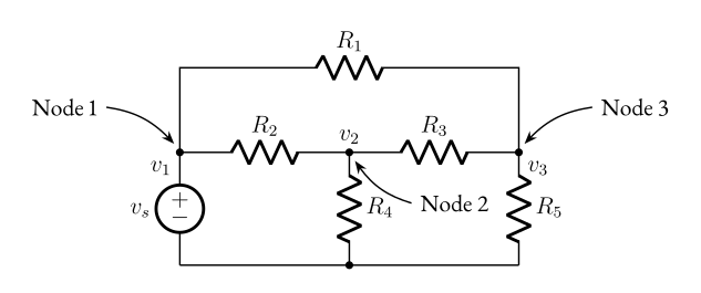
We can try all we want to simplify it, with our current knowledge, we simply can’t.

So let’s learn about Node-Voltage analysis.

Node-Voltage analysis

Below is a picture that illustrates the idea:

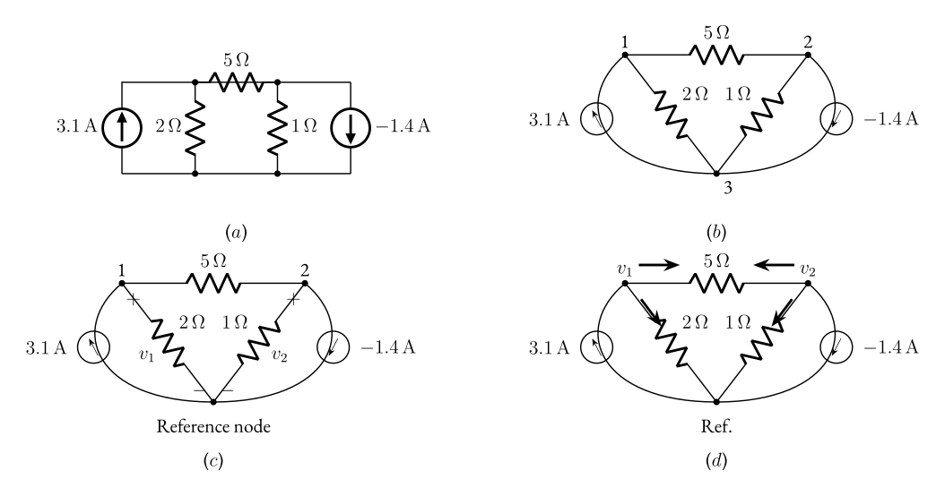
Here’s the idea:

Algorithm 1: Node-voltage analysis

Find the nodes
Assign a reference node (usually, we pick the node with most connections)
Assign node voltages (Note, in a circuit with, $N$ , nodes we have, $N - 1$ , voltages)
Then we solve these using KCL on each node ( $\sum i_{out} = \sum i_{in}$ )

The convention is also the following:

Consider $i_{out}$ in resistors
Consider $i_{out}$ as positive
$V_{\text{current}} - V_{\text{adjacent}}$

So, if we solve the example we get:

Using KCL on the first node,

\frac{v_1}{2} + \frac{v_1 - v_2}{5} = 3.1.

For the second node,

\frac{v_2}{1} + \frac{v_2 - v_1}{5} = -(-1.4).

Solving for $v_1$ and $v_2$ we get,

v_1 = 5\,\mathrm{V}, \quad v_2 = 2\,\mathrm{V}.

Notice that we can do this in a matrix form as well,

\begin{bmatrix} 0.7 & -0.2 \newline -0.2 & 1.2 \end{bmatrix} \begin{bmatrix} v_1 \newline v_2 \end{bmatrix} = \begin{bmatrix} 3.1 \newline 1.4 \end{bmatrix}.

Supernode

Voltage source between nodes that are not the reference node.

Solution: we treat it as one node.

Mesh-Current analysis

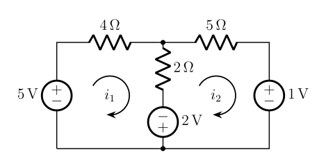
Is the opposite of Node-voltage analysis. Therefore, we just apply KVL instead of KCL. Note that this only works for planar circuits.

Definition 1 (Planar circuit)

It is possible to draw it in a plane without crossing wires.

Example:

\begin{align*} -5 + 4i_1 + 2(i_1 - i_2) - 2 & = 0, \newline 2 + 2(i_2 - i_1) + 5i_2 + 1 & = 0. \end{align*}

Supermesh

Same principle as super node but for the mesh-current.

Superposition

Theorem 1 (Superposition)

As the name suggests, it’s the principle that, given a linear system, the net response caused by two or more stimuli is the sum of these responses.

In our case, the stimuli are voltage/current sources.

So our method is:

Algorithm 2: Superposition

Leave one source ON and turn all other sources OFF.
- Voltage sources: $v = 0$ , these become short circuits.
- Current sources: $i = 0$ , these become open circuits.
Add the resulting responses to find the total response.

Example:

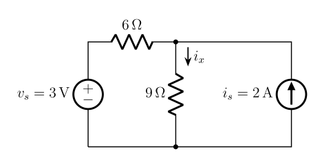
Let’s call the circuit when we turn off the current source for $i^\prime_{x}$ , and the circuit when we turn off the voltage source for $i^{\prime \prime}_{x}$ .

The circuit for $i^\prime_x$ becomes:

Figure 5: The current source turned off.

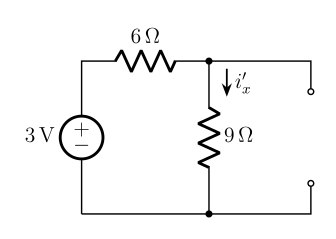
We can easily solve this:

\begin{align*} V & = R \cdot I, \newline 3\,\mathrm{V} & = R_{eq} \cdot i^{\prime}_{x}, \newline i^\prime_x & = \frac{3\,\mathrm{V}}{6\,\Omega + 9\,\Omega} = 0.2\,\mathrm{A}. \end{align*}

The circuit for $i^{\prime \prime}_x$ becomes:

Figure 6: The voltage source turned off.

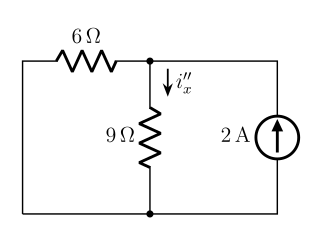
We can solve this by,

\begin{align*} R_{eq} & = \frac{R_1 R_2}{R_1 + R_2}, \newline V & = i_{\text{total}} \cdot R_{eq}, \end{align*}

i_x^{\prime \prime} = \frac{V}{R_{i^{\prime \prime}_x}},

\begin{align*} i_x^{\prime \prime} & = i_{\text{total}} \cdot \frac{R_6}{R_6 + R_{i^{\prime \prime}_x}} \newline & = 2\,\mathrm{A} \cdot \frac{6\,\Omega}{6\,\Omega + 9\,\Omega} = 0.8\,\mathrm{A}. \end{align*}

Finally, using the actual superposition principle,

i_x = i^\prime_x + i^{\prime \prime}_x = 0.2\,\mathrm{A} + 0.8\,\mathrm{A} = \boxed{1.0\,\mathrm{A}}.

Equivalent circuits

When dealing with complex circuits, like the one we encountered earlier, with our current knowledge it takes a lot of time and effort to simplify circuits.

Luckily, there’s a more powerful method to find equivalent circuits.

It’s called the Thévenin equivalent circuits and Norton equivalent circuits.

The idea is the following:

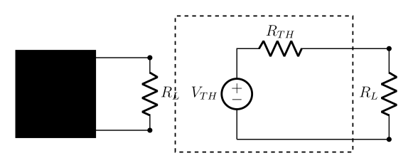
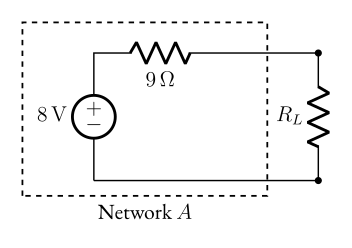
Figure 7: A complex network and its Thévenin equivalent.

We take a complex network and transform it to just a single voltage source and resistor.

These are called the Thévenin voltage and resistance. We’ll see later why we’ll want to name these.

But how do we actually do this transformation?

Algorithm 3: Thévenin equivalent

Disconnect the “load”, $R_L$ .
Find the open circuit voltage, $V_{oc}$ .
Find the equivalent resistance, $R_{eq}$ , of the network with all independent sources turned off.
Then:
- $V_{TH} = V_{oc}$
- $R_{TH} = R_{eq}$

Example:

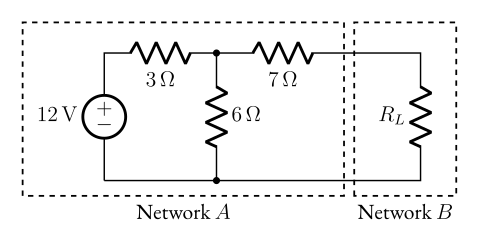
Let’s now disconnect $R_L$ and find the open circuit voltage:

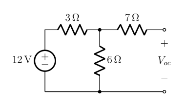
\begin{align*} V_{oc} & = V_6 \quad \text{(since they are in parallel)}, \newline V_6 & = V_{\text{total}} \cdot \frac{R_6}{R_3 + R_6} = 12\,\mathrm{V} \cdot \frac{6\,\Omega}{3\,\Omega + 6\,\Omega} = 8\,\mathrm{V}, \newline V_{TH} & = V_{oc} = 8\,\mathrm{V}. \end{align*}

Notice how we didn’t include the $R_7$ , this is due to the fact that, no current is going through that resistor!

Next step, let’s find the $R_{eq}$ for this circuit. Don’t forget to turn OFF all independent sources!:

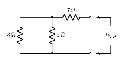
Figure 10: The equivalent resistance with the source turned off.

\begin{align*} R_{eq} & = R_{3 \| 6} + R_7 = 2\,\Omega + 7\,\Omega = 9\,\Omega, \newline R_{TH} & = R_{eq} = 9\,\Omega. \end{align*}

Therefore, the final equivalent circuit is:

Figure 11: The Thévenin equivalent circuit.

Norton equivalent circuits

Norton equivalent is the same idea, but we replace the voltage source with a current source, and make the resistors parallel instead:

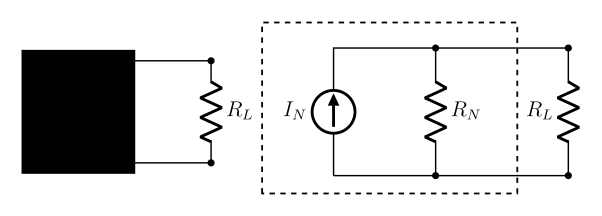
Figure 12: A complex network and its Norton equivalent.

The method for finding a Norton equivalent circuit is:

Algorithm 4: Norton equivalent

Replace the load with a short circuit.
Find the short circuit current, $I_{sc}$ .
Find the equivalent resistance, $R_{eq}$ , of the network with all independent sources turned off.
Then:
- $I_N = I_{sc}$
- $R_N = R_{eq}$

Source transformation

Now comes the beauty with all of this, we can transform a Thévenin equivalent circuit to a Norton equivalent circuit!

It’s quite obvious because,

R_{TH} = R_{N} = R_{eq}.

But the beauty is,

V_{TH} = I_{N} \cdot R_{eq}.

Using Ohm’s law, we can easily just convert one type of circuit to the corresponding other type!

We’ll be using this tool a lot in the future for analyzing circuits!