Part 5 - Electrical fields

In this part we’ll discuss electrical fields and some tools we’ll begin to use.

So far we’ve only analyzed the electrical circuits at a macro level. In this part we’ll try to dissect them at a micro-level, so let’s zoom in!

Electrical charge

To understand electrical circuits, let’s first understand electrical charge.

As we’ve seen, we use $q$ , as the notation for charge. The elementary charge (the charge carried by a single proton) is:

e = 1.602 \cdot 10^{-19} \ \mathrm{C}.

We also need to remember this very important law:

Theorem 1 (Conservation of charge)

The total charge within a closed system cannot change. It can only be redistributed.

Now that we’ve defined electrical charge, we can define electrical fields!

Electrical fields

Let’s start by defining what an electrical field is!

Definition 1 (Electrical field)

An electrical field is a force field created by electric charges.

Always remember:

Repulsive if charges are the same.
Attractive if charges are different.

Coulomb’s law

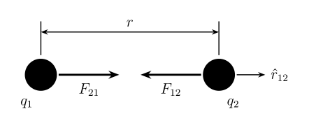
Figure 1: Two charges and the forces between them.

This force field that is created by the charges, we can mathematically compute these forces:

Theorem 2 (Coulomb’s law)

\vec{\mathbf{F}}_{12} = k_e \frac{q_1 q_2}{r^2} \hat{\mathbf{r}}_{12},

where $k_e$ is Coulomb’s constant,

k_e = \frac{1}{4\pi\varepsilon_0}.

Where $\varepsilon_0$ is the vacuum permittivity, we’ll actually derive this later on!

\varepsilon_0 \approx \frac{10^{-9}}{36\pi} \ \mathrm{F/m}.

Alright with all of these tools, we can finally define electrical fields with some maths!

\vec{\mathbf{E}} = k_e \frac{q}{r^2} \hat{\mathbf{r}}.

Also, given an electrical field we can calculate the force on a point of charge,

\vec{\mathbf{F}}_E = q \vec{\mathbf{E}}.

Notice how these formulas are really similar to formulas of gravitation.

Superposition

As you could have guessed, yes, the superposition principle applies to the electrical forces and fields,

\begin{align*} \vec{\mathbf{F}}_j & = \sum_{i = 1}^{N} \vec{\mathbf{F}}_{ij}, \newline \vec{\mathbf{E}} & = \sum_{i = 1}^{N} \vec{\mathbf{E}}_i. \end{align*}

Dipoles

Definition 2 (Dipole)

Two equal and opposite charges are known as a dipole.

A dipole moment is a measure of the density of the electrical field of a dipole.

The formula,

\vec{\mathbf{p}} = q \vec{\mathbf{d}},

where $\vec{\mathbf{d}}$ is the direction vector, which is defined as, from negative charge to positive charge by convention.

This means, placing a dipole in an electrical field, applies a torque on the dipole:

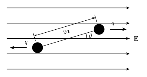
Figure 2: A dipole in a uniform electrical field.

Which means we can calculate the torque,

\begin{align*} \vec{\boldsymbol{\tau}} & = \vec{\mathbf{p}} \times \vec{\mathbf{E}}, \newline \tau & = p E \sin(\theta). \end{align*}

Electrical flux

So far we’ve discussed a discrete number of charges and points. Imagine now instead that we have a continuous line:

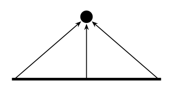
Figure 3: The field from a continuous line of charge at a point.

So instead of,

\vec{\mathbf{E}} = \sum_{i = 1}^{N} \vec{\mathbf{E}}_i,

we get,

\vec{\mathbf{E}} = \int_{L_1}^{L_2} \vec{\mathbf{E}}_l \, dl.

Now, let’s flip it around. We instead have a single point of charge and want to know how much of its electrical field passes through a line.

This is precisely electrical flux! We denote electrical flux with $\Phi$ .

\Phi = \sum_{i = 1}^{N} \vec{\mathbf{E}}_i \cdot \hat{n}.

And for the continuous case,

\Phi = \int_{L_1}^{L_2} \vec{\mathbf{E}}_l \cdot \hat{n} \, dl.

Let’s now add another dimension, so it’s a surface.

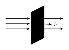
Field lines passing through a surface with normal \hat{n}. — Figure 4: Field lines passing through a surface with normal $\hat{n}$ .

\Phi = \iint \vec{\mathbf{E}} \cdot \hat{n} \, dA = \iint E \, dA \cos(\theta).

If we’re instead within a closed contour:

Figure 5: A point charge inside a closed surface.

For this we use the special integral symbol,

\Phi = \oiint \vec{\mathbf{E}} \cdot d\vec{\mathbf{A}}.

What is the total flux through this surface (circle)?

\begin{align*} E & = \frac{q}{4\pi r^2 \varepsilon_0}, \newline A & = 4\pi r^2. \end{align*}

Therefore,

\Phi = \frac{q}{4\pi r^2 \varepsilon_0} 4\pi r^2 = \frac{q}{\varepsilon_0}.

Gauss’s law

This is Gauss’s law!

Theorem 3 (Gauss’s law)

\Phi_E = \oiint \vec{\mathbf{E}} \cdot d\vec{\mathbf{A}} = \frac{q}{\varepsilon_0}

Gaussian surfaces

Since this is from a specific surface, we’ll need to consider the different types:

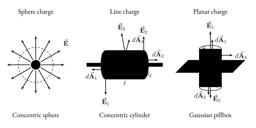
These are the gaussian surfaces that we’ll be looking into!