In this part we’ll work in electrical fields, the connection between electrical fields and voltages as well as how we can use electrical fields with capacitors.
Work
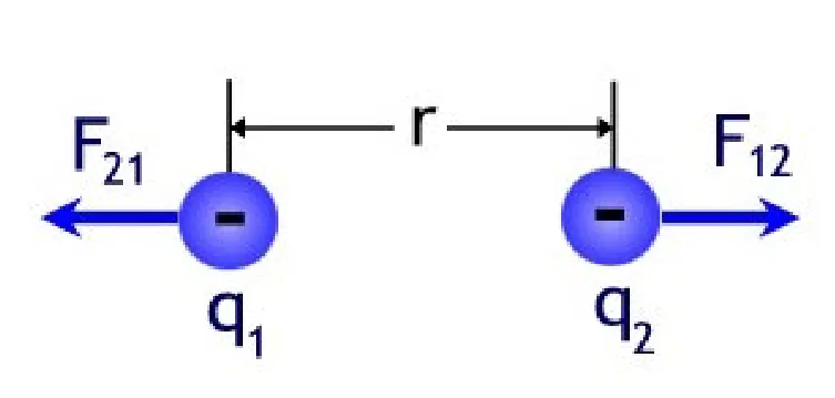
We’ve briefly went over work before in this series - but let’s consider the work required to move charges apart from eachother.
Note, in the case when we move perpendicular to the field, the work is 0.
Another way we can write work is:
W=ΔU=−∫ABF⋅dr
This means that the potential is proportional to the charge:
FE=qE
If we normalize the work with the charge we’ll see a very interesting result:
qW=−∫ABE⋅dr
If we just interpret this integral, we move a charged particle a distance.
Let’s go back to our definition of voltage from the first part - this is precisely the difference in voltage!
[ΔV]=CoulumbJoules
Just as Kirchoff’s voltage law tells us that, within a closed loop, the sum of the voltages are 0.
This means that the work done within a closed path:
W=−∮F⋅dr=0
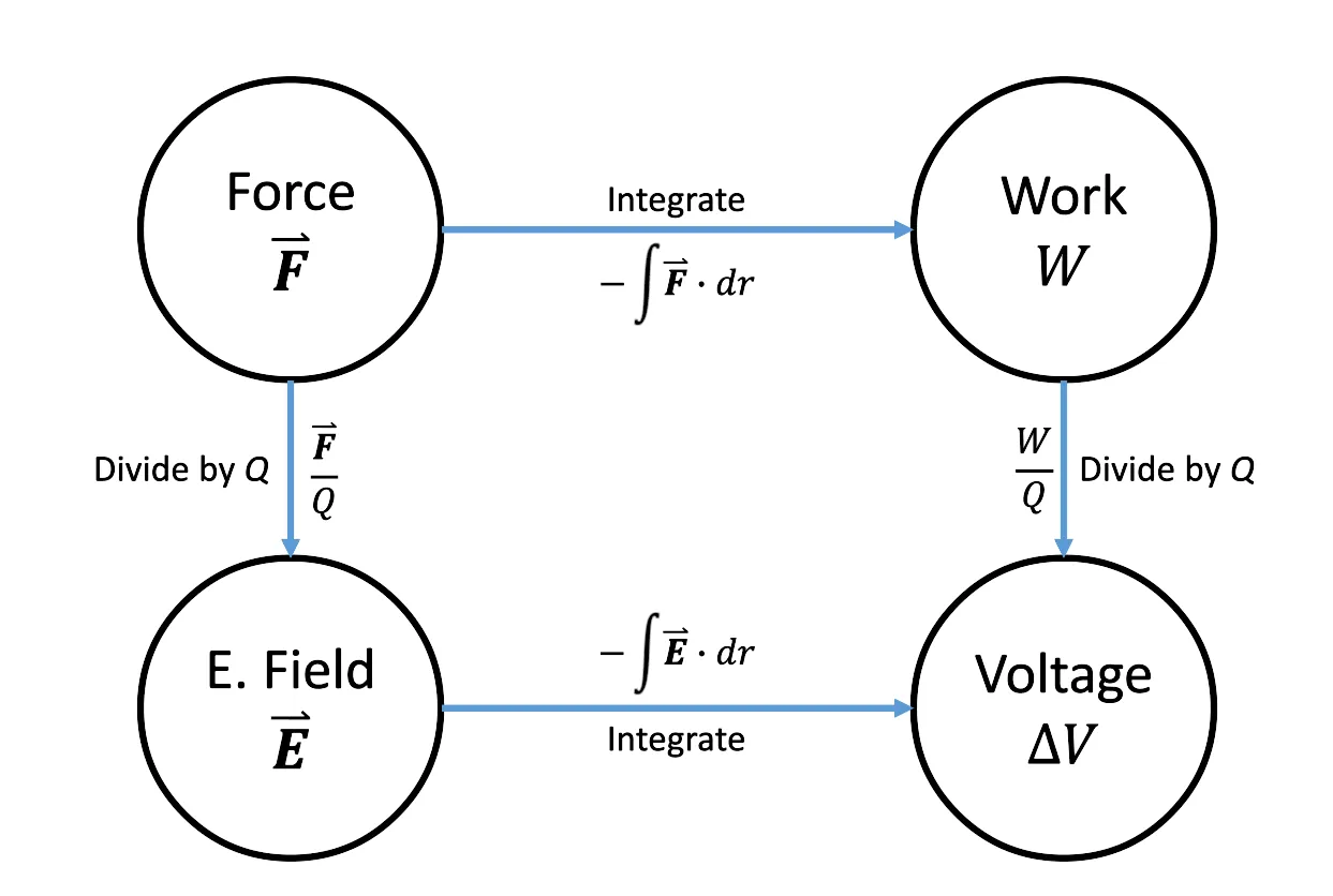
With all these new formulas, here is a little cheat sheet so that we remember:
Electrical fields
If we work backwards from a known voltage - we can find the electrical field!
ΔV=−∫ABE⋅drdV=−E⋅drE=−drdV
We can define this as the gradient of the voltage:
E=−∇V
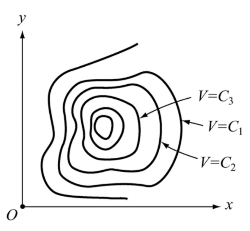
Equipotential curves
As we just discovered - the electrical field is equal to the gradient of the voltage.
Equipotential curves are way of visualizing the electric potential in a region of space.
They are just like geographical maps!
Now the interesting part is that these curves are always perpendicular to the electrical field lines!
Capacitance
Capacitance is the ability for an electrical potential to hold a charge
We define capacitance as:
C=∣ΔV∣q
Capacitors
Capacitors are two isolated plates with equal and opposite charges: ±q
When they are charged, they create a voltage diffrence between the plates, naturally.
How can we calculate this voltage?
Assume we have a surface area of A, a surface charge density of σ.
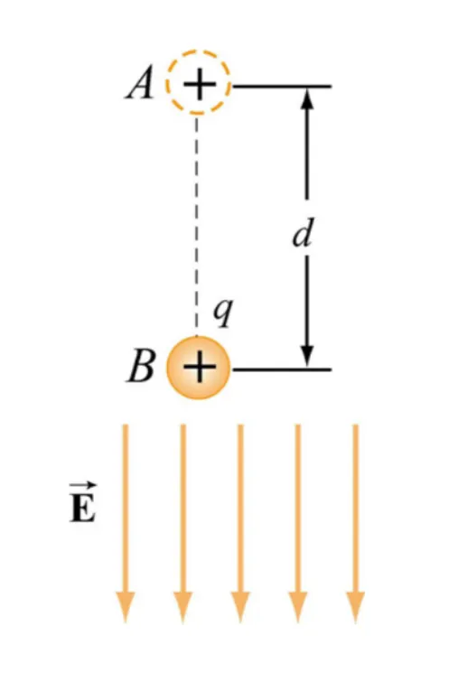 Let’s calculate the work to move from A to B.