Dynamic systems
u ( t ) u(t) u ( t )
y ( t ) y(t) y ( t )
We usually represent our systems with ODEs of the form:
y ˙ + a y = b u \dot{y} + ay = bu y ˙ + a y = b u Feedback systems
Using (positive or negative) feedback, meaning our input depends on the output as well!
r ( t ) r(t) r ( t )
e ( t ) e(t) e ( t ) r ( t ) − y ( t ) r(t) - y(t) r ( t ) − y ( t )
Laplace Domain
F ( s ) F(s) F ( s )
G u y ( s ) G_{uy}(s) G u y ( s ) Y ( s ) U ( s ) \dfrac{Y(s)}{U(s)} U ( s ) Y ( s )
L ( s ) = G u y ( s ) F ( s ) L(s) = G_{uy}(s) F(s) L ( s ) = G u y ( s ) F ( s )
G r y ( s ) G_{ry}(s) G r y ( s ) Y ( s ) R ( s ) = L ( s ) 1 + L ( s ) \dfrac{Y(s)}{R(s)} = \dfrac{L(s)}{1 + L(s)} R ( s ) Y ( s ) = 1 + L ( s ) L ( s )
Poles & Zeroes
Poles are given by 1 + L ( s ) = 0 1 + L(s) = 0 1 + L ( s ) = 0 G r y ( s ) G_{ry}(s) G r y ( s )
Zeroes are given by L ( s ) = 0 L(s) = 0 L ( s ) = 0 G r y ( s ) G_{ry}(s) G r y ( s )
Controllers
P-controller
u ( t ) = K p ⋅ e ( t ) u(t) = K_p \cdot e(t) u ( t ) = K p ⋅ e ( t ) U ( s ) = K p ⋅ E ( s ) U(s) = K_p \cdot E(s) U ( s ) = K p ⋅ E ( s ) PI-controller
u ( t ) = K p ⋅ e ( t ) + K i ∫ 0 t e ( τ ) d τ u(t) = K_p \cdot e(t) + K_i \int_0^t e(\tau)\ d\tau u ( t ) = K p ⋅ e ( t ) + K i ∫ 0 t e ( τ ) d τ U ( s ) = K p ⋅ E ( s ) + K i s ⋅ E ( s ) U(s) = K_p \cdot E(s) + \frac{K_i}{s} \cdot E(s) U ( s ) = K p ⋅ E ( s ) + s K i ⋅ E ( s ) PD-controller
u ( t ) = K p ⋅ e ( t ) + K d ⋅ d ( e ( t ) ) d t u(t) = K_p \cdot e(t) + K_d \cdot \dfrac{d(e(t))}{dt} u ( t ) = K p ⋅ e ( t ) + K d ⋅ d t d ( e ( t )) U ( s ) = K p ⋅ E ( s ) + s K d ⋅ E ( s ) U(s) = K_p \cdot E(s) + sK_d \cdot E(s) U ( s ) = K p ⋅ E ( s ) + s K d ⋅ E ( s ) PID-controller
u ( t ) = K p ⋅ e ( t ) + K i ∫ 0 t e ( τ ) d τ + K d ⋅ d ( e ( t ) ) d t u(t) = K_p \cdot e(t) + K_i \int_0^t e(\tau)\ d\tau + K_d \cdot \dfrac{d(e(t))}{dt} u ( t ) = K p ⋅ e ( t ) + K i ∫ 0 t e ( τ ) d τ + K d ⋅ d t d ( e ( t )) U ( s ) = K p ⋅ E ( s ) + K i s ⋅ E ( s ) + s K d ⋅ E ( s ) U(s) = K_p \cdot E(s) + \frac{K_i}{s} \cdot E(s) + sK_d \cdot E(s) U ( s ) = K p ⋅ E ( s ) + s K i ⋅ E ( s ) + s K d ⋅ E ( s ) Feedback systems with noise/disturbance
Remaining control error, e ( ∞ ) e(\infty) e ( ∞ )
r ( t ) = r 0 ⋅ σ ( t ) r(t) = r_0 \cdot \sigma(t) r ( t ) = r 0 ⋅ σ ( t ) R ( s ) = r 0 s ∣ set v ( t ) = 0 R(s) = \dfrac{r_0}{s} \ | \ \text{set } v(t) = 0 R ( s ) = s r 0 ∣ set v ( t ) = 0 lim t → ∞ e ( t ) = lim s → 0 s ⋅ E ( s ) = lim s → 0 s ⋅ ( R ( s ) − L ( s ) 1 + L ( s ) R ( s ) ) = lim s → 0 s ⋅ ( R ( s ) ⋅ ( 1 − L ( s ) 1 + L ( s ) ) ) = lim s → 0 s ⋅ ( R ( s ) ⋅ ( 1 + L ( s ) − L ( s ) 1 + L ( s ) ) ) = lim s → 0 s ⋅ ( R ( s ) ⋅ ( 1 1 + L ( s ) ) ) = lim s → 0 s ⋅ ( r 0 s ⋅ 1 1 + L ( s ) ) = lim s → 0 ( r 0 1 + L ( 0 ) ) = lim s → 0 ( r 0 1 + F ( 0 ) G ( 0 ) ) \begin{align*}
\lim_{t \to \infty} e(t)
& = \lim_{s \to 0} s \cdot E(s) \newline
& = \lim_{s \to 0} s \cdot \left(R(s) - \dfrac{L(s)}{1 + L(s)} R(s)\right) \newline
& = \lim_{s \to 0} s \cdot \left(R(s) \cdot \left(1 - \dfrac{L(s)}{1 + L(s)}\right)\right) \newline
& = \lim_{s \to 0} s \cdot \left(R(s) \cdot \left(\dfrac{1 + L(s) - L(s)}{1 + L(s)}\right)\right) \newline
& = \lim_{s \to 0} s \cdot \left(R(s) \cdot \left(\dfrac{1}{1 + L(s)}\right)\right) \newline
& = \lim_{s \to 0} s \cdot \left(\dfrac{r_0}{s} \cdot \dfrac{1}{1 + L(s)}\right) \newline
& = \lim_{s \to 0} \left(\dfrac{r_0}{1 + L(0)}\right) \newline
& = \boxed{\lim_{s \to 0} \left(\dfrac{r_0}{1 + F(0)G(0)}\right)}
\end{align*} t → ∞ lim e ( t ) = s → 0 lim s ⋅ E ( s ) = s → 0 lim s ⋅ ( R ( s ) − 1 + L ( s ) L ( s ) R ( s ) ) = s → 0 lim s ⋅ ( R ( s ) ⋅ ( 1 − 1 + L ( s ) L ( s ) ) ) = s → 0 lim s ⋅ ( R ( s ) ⋅ ( 1 + L ( s ) 1 + L ( s ) − L ( s ) ) ) = s → 0 lim s ⋅ ( R ( s ) ⋅ ( 1 + L ( s ) 1 ) ) = s → 0 lim s ⋅ ( s r 0 ⋅ 1 + L ( s ) 1 ) = s → 0 lim ( 1 + L ( 0 ) r 0 ) = s → 0 lim ( 1 + F ( 0 ) G ( 0 ) r 0 ) Remaining control error, e ( ∞ ) e(\infty) e ( ∞ )
v ( t ) = v 0 ⋅ σ ( t ) v(t) = v_0 \cdot \sigma(t) v ( t ) = v 0 ⋅ σ ( t ) V ( s ) = v 0 s ∣ set r ( t ) = 0 V(s) = \dfrac{v_0}{s} \ | \ \text{set } r(t) = 0 V ( s ) = s v 0 ∣ set r ( t ) = 0 E ( s ) = R ( s ) − Y ( s ) E(s) = R(s) - Y(s) \newline E ( s ) = R ( s ) − Y ( s ) E ( s ) = − Y ( s ) E(s) = -Y(s) \newline E ( s ) = − Y ( s ) E ( s ) = − ( G ( s ) ⋅ ( V ( s ) + F ( s ) E ( s ) ) ) E(s) = -\left(G(s) \cdot \left(V(s) + F(s) E(s)\right)\right) \newline E ( s ) = − ( G ( s ) ⋅ ( V ( s ) + F ( s ) E ( s ) ) ) E ( s ) = − G ( s ) V ( s ) − L ( s ) E ( s ) E(s) = -G(s) V(s) - L(s) E(s) \newline E ( s ) = − G ( s ) V ( s ) − L ( s ) E ( s ) E ( s ) + L ( s ) E ( s ) = − G ( s ) V ( s ) E(s) + L(s) E(s) = -G(s) V(s) \newline E ( s ) + L ( s ) E ( s ) = − G ( s ) V ( s ) E ( s ) ( 1 + L ( s ) ) = − G ( s ) V ( s ) E(s) \left(1 + L(s)\right) = -G(s) V(s) \newline E ( s ) ( 1 + L ( s ) ) = − G ( s ) V ( s ) E ( s ) = − G ( s ) V ( s ) 1 + L ( s ) E(s) = -\dfrac{G(s) V(s)}{1 + L(s)} \newline E ( s ) = − 1 + L ( s ) G ( s ) V ( s ) E ( s ) = − G ( s ) 1 + L ( s ) ⋅ V ( s ) E(s) = -\dfrac{G(s)}{1 + L(s)} \cdot V(s) \newline E ( s ) = − 1 + L ( s ) G ( s ) ⋅ V ( s ) lim t → ∞ e ( t ) = lim s → 0 s ⋅ E ( s ) = lim s → 0 s ⋅ − G ( s ) 1 + L ( s ) ⋅ V ( s ) = lim s → 0 s ⋅ − G ( s ) 1 + L ( s ) ⋅ v 0 s = lim s → 0 − G ( s ) ⋅ v 0 1 + L ( s ) = lim s → 0 − G ( 0 ) ⋅ v 0 1 + L ( 0 ) \begin{align*}
\lim_{t \to \infty} e(t)
& = \lim_{s \to 0} s \cdot E(s) \newline
& = \lim_{s \to 0} s \cdot -\dfrac{G(s)}{1 + L(s)} \cdot V(s) \newline
& = \lim_{s \to 0} s \cdot -\dfrac{G(s)}{1 + L(s)} \cdot \dfrac{v_0}{s} \newline
& = \lim_{s \to 0} -\dfrac{G(s) \cdot v_0}{1 + L(s)} \newline
& = \boxed{\lim_{s \to 0} -\dfrac{G(0) \cdot v_0}{1 + L(0)}}
\end{align*} t → ∞ lim e ( t ) = s → 0 lim s ⋅ E ( s ) = s → 0 lim s ⋅ − 1 + L ( s ) G ( s ) ⋅ V ( s ) = s → 0 lim s ⋅ − 1 + L ( s ) G ( s ) ⋅ s v 0 = s → 0 lim − 1 + L ( s ) G ( s ) ⋅ v 0 = s → 0 lim − 1 + L ( 0 ) G ( 0 ) ⋅ v 0 To eliminate the remaining control error all together, meaning that e ( ∞ ) = 0 e(\infty) = 0 e ( ∞ ) = 0 F ( 0 ) = ∞ F(0) = \infty F ( 0 ) = ∞ 1 s \frac{1}{s} s 1
Physical models
Physical models are often model with ODEs, for example:
m y ¨ ( t ) = F ( t ) − k y ( t ) − b y ˙ ( t ) m\ddot{y}(t) = F(t) - ky(t) - b\dot{y}(t) m y ¨ ( t ) = F ( t ) − k y ( t ) − b y ˙ ( t ) m y ¨ ( t ) + b y ˙ ( t ) + k y ( t ) = F ( t ) m\ddot{y}(t) + b\dot{y}(t) + ky(t) = F(t) m y ¨ ( t ) + b y ˙ ( t ) + k y ( t ) = F ( t ) Taking the Laplace transform
m s 2 Y ( s ) + b s Y ( s ) + k Y ( s ) = L F ( s ) ms^2 Y(s) + bs Y(s) + kY(s) \stackrel{\mathcal{L}}{=} F(s) m s 2 Y ( s ) + b s Y ( s ) + k Y ( s ) = L F ( s ) Y ( s ) ( m s 2 + b s + k ) = F ( s ) Y(s) \left(ms^2 + bs + k\right) = F(s) Y ( s ) ( m s 2 + b s + k ) = F ( s ) G ( s ) = F ( s ) ( m s 2 + b s + k ) \boxed{G(s) = \dfrac{F(s)}{\left(ms^2 + bs + k\right)}} G ( s ) = ( m s 2 + b s + k ) F ( s ) We can also do this with state-space representation.
Rewriting our original ODE:
y ¨ ( t ) = − b m y ˙ ( t ) − k m y ( t ) + 1 m F ( t ) \ddot{y}(t) = -\frac{b}{m} \dot{y}(t) - \frac{k}{m} y(t) + \frac{1}{m} F(t) y ¨ ( t ) = − m b y ˙ ( t ) − m k y ( t ) + m 1 F ( t ) Let x 1 = y x_1 = y x 1 = y x 2 = y ˙ x_2 = \dot{y} x 2 = y ˙
This means that:
{ x 1 ˙ = x 2 x 2 ˙ = − b m x 2 − k m x 1 + 1 m F \begin{cases}
\dot{x_1} & = x_2 \newline
\dot{x_2} & = -\dfrac{b}{m} x_2 - \dfrac{k}{m} x_1 + \dfrac{1}{m} F
\end{cases} ⎩ ⎨ ⎧ x 1 ˙ x 2 ˙ = x 2 = − m b x 2 − m k x 1 + m 1 F Using Matrix notation:
x = [ x 1 ˙ x 2 ˙ ] = [ 0 1 − k m − b m ] [ x 1 x 2 ] + [ 0 1 m ] F x =
\begin{bmatrix}
\dot{x_1} \newline
\dot{x_2}
\end{bmatrix} =
\begin{bmatrix}
0 & 1 \newline
-\frac{k}{m} & -\frac{b}{m}
\end{bmatrix}
\begin{bmatrix}
x_1 \newline
x_2
\end{bmatrix} +
\begin{bmatrix}
0 \newline
\frac{1}{m}
\end{bmatrix} F x = [ x 1 ˙ x 2 ˙ ] = [ 0 − m k 1 − m b ] [ x 1 x 2 ] + [ 0 m 1 ] F y = [ 1 0 ] [ x 1 x 2 ] + [ 0 ] F y =
\begin{bmatrix}
1 & 0
\end{bmatrix}
\begin{bmatrix}
x_1 \newline
x_2
\end{bmatrix} +
\begin{bmatrix}
0
\end{bmatrix}
F y = [ 1 0 ] [ x 1 x 2 ] + [ 0 ] F Generalization
x ˙ = A x + B u y = C x + D u \dot{x} = Ax + Bu \newline
y = Cx + Du x ˙ = A x + B u y = C x + D u G u y ( s ) = Y ( s ) U ( s ) = C ( s I − A ) − 1 B + D G_{uy}(s) = \dfrac{Y(s)}{U(s)} = C(sI - A)^{-1} B + D G u y ( s ) = U ( s ) Y ( s ) = C ( s I − A ) − 1 B + D Characteristics equation
To find the poles of the system in matrix notation we use the fact that the denominator of the transfer function is:
d e t ( s I − A ) det(sI - A) d e t ( s I − A ) So, to find the poles we simply:
d e t ( s I − A ) = 0 det(sI - A) = 0 d e t ( s I − A ) = 0 Reminder that:
A = [ a b c d ] A =
\begin{bmatrix}
a & b \newline
c & d
\end{bmatrix} A = [ a c b d ] d e t ( A ) = 1 a d − b c det(A) =
\dfrac{1}{ad - bc} d e t ( A ) = a d − b c 1 A − 1 = 1 a d − b c [ d − b − c a ] A^{-1} =
\dfrac{1}{ad - bc}
\begin{bmatrix}
d & -b \newline
-c & a
\end{bmatrix} A − 1 = a d − b c 1 [ d − c − b a ] NB: This rule only applies for 2x2 matrices.
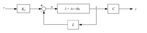
State feedback
u = K r ⋅ r − L x y = C x u = K_r \cdot r - Lx \newline
y = Cx u = K r ⋅ r − Lx y = C x x ˙ = A x + B u = A x + B ( K r r − L x ) s X ( s ) = A X ( s ) + B ( K r R ( s ) − L X ( s ) ) s X ( s ) = A X ( s ) + B K r R ( s ) − B L X ( s ) s X ( s ) − A X ( s ) + B L X ( s ) = B K r R ( s ) X ( s ) ( s I − A + B L ) = B K r R ( s ) X ( s ) = ( s I − A + B L ) − 1 B K r R ( s ) \dot{x} = Ax + Bu = Ax + B(K_r r - Lx) \newline
sX(s) = AX(s) + B(K_r R(s) - LX(s)) \newline
sX(s) = AX(s) + BK_r R(s) - BLX(s) \newline
sX(s) - AX(s) + BLX(s) = BK_r R(s) \newline
X(s) (sI - A + BL) = BK_r R(s) \newline
X(s) = (sI - A + BL)^{-1} BK_r R(s) \newline x ˙ = A x + B u = A x + B ( K r r − Lx ) s X ( s ) = A X ( s ) + B ( K r R ( s ) − L X ( s )) s X ( s ) = A X ( s ) + B K r R ( s ) − B L X ( s ) s X ( s ) − A X ( s ) + B L X ( s ) = B K r R ( s ) X ( s ) ( s I − A + B L ) = B K r R ( s ) X ( s ) = ( s I − A + B L ) − 1 B K r R ( s ) Y ( s ) = C X ( s ) Y ( s ) = C ( s I − A + B L ) − 1 B K r R ( s ) G r y s = Y ( s ) R ( s ) = C ( s I − A + B L ) − 1 B K r Y(s) = CX(s) \newline
Y(s) = C (sI - A + BL)^{-1} B K_r R(s) \newline
G_{ry}{s} = \dfrac{Y(s)}{R(s)} = C (sI - A + BL)^{-1} B K_r Y ( s ) = C X ( s ) Y ( s ) = C ( s I − A + B L ) − 1 B K r R ( s ) G r y s = R ( s ) Y ( s ) = C ( s I − A + B L ) − 1 B K r We can determine K_r for a system with the knowledge that G ( 0 ) = 1 G(0) = 1 G ( 0 ) = 1
So:
K r = 1 C ( − A + B L ) − 1 ) B K_r = \dfrac{1}{C(-A + BL)^{-1}) B} K r = C ( − A + B L ) − 1 ) B 1 Poles are given by:
d e t ( s I − A + B L ) = 0 det(sI - A + BL) = 0 d e t ( s I − A + B L ) = 0 Stability
A system is stable if and only if its characteristic equation has roots in the LHP, meaning that ℜ ( s ) < 0 \Re(s) < 0 ℜ ( s ) < 0
For systems of order 2, this means that all the coefficients are > 0 > 0 > 0
For systems or order 3 or higher we use Routh–Hurwitz method.
Nyquists simplified criterion
To use the Nyquists simplified criterion, L ( s ) L(s) L ( s ) L ( j ω ) L(j\omega) L ( j ω ) 0 ≤ ω ≤ ∞ 0 \leq \omega \leq \infty 0 ≤ ω ≤ ∞
If L ( j ω ) L(j\omega) L ( j ω ) ( − 1 , 0 ) (-1, 0) ( − 1 , 0 )
Nyquists criterion
If L ( s ) L(s) L ( s )
Z = P + N = Number of zeroes 1 + L ( s ) has in RHP. Z = P + N = \text{Number of zeroes } 1 + L(s) \text{ has in RHP.} Z = P + N = Number of zeroes 1 + L ( s ) has in RHP. P = Number of poles L ( s ) has in RHP. P = \text{Number of poles } L(s) \text{ has in RHP.} P = Number of poles L ( s ) has in RHP. N = Number of turns L ( j ω ) has around ( − 1 , 0 ) clockwise. N = \text{Number of turns } L(j\omega) \text{ has around } (-1, 0) \text{ clockwise.} N = Number of turns L ( j ω ) has around ( − 1 , 0 ) clockwise.