Part 6 - State Space Approach

Introduction

In this part, we will be discussing the state space approach to modeling systems. This approach is a powerful tool that allows us to model systems in a way that is independent of the input and output signals. This makes it easier to analyze and design control systems for complex systems.

This is a “modern” approach to modeling systems, as opposed to the “classical” approach that we have been using so far. The state space approach is more general and can be used to model a wide range of systems, including systems with multiple inputs and outputs.

We’ll derive a linear state space equation,

From a higher order ODE or transfer function.
From physical laws.
From the Jacobian linearization of nonlinear systems.

State Space Approach

When we are modeling a set of first order $n$ -dimensional ODEs,

\begin{aligned} \dot{x} & = f(x, u, t) \newline y & = h(x, u, t) \newline x(0) & = x_0, t \geq 0. \end{aligned}

where,

\begin{aligned} f(x, u, t) & = \begin{bmatrix} f_1(x, u, t) \newline f_2(x, u, t) \newline \vdots \newline f_n(x, u, t) \end{bmatrix} \in \mathbb{R}^n \newline h(x, u, t) & = \begin{bmatrix} h_1(x, u, t) \newline h_2(x, u, t) \newline \vdots \newline h_m(x, u, t) \end{bmatrix} \in \mathbb{R}^p. \end{aligned}

$x = [x_1, x_2, \ldots, x_n]^T \in \mathbb{R}^n$ is called the state of the system (the component of x can stand for position, velocity, voltage and current).

$u = [u_1, u_2, \ldots, u_m]^T \in \mathbb{R}^m$ is called the input of the system.

$y = [y_1, y_2, \ldots, y_p]^T \in \mathbb{R}^p$ is called the output of the system, and $n$ is called the dimension or the order of the system.

Remark: When $m = p = 1$ , single input, single output, we have a SISO system.

When $m > 1 or p > 1$ , multi input, multi output, we have a MIMO system.

When $f$ and $h$ do not explicitly depend on $t$ , that is,

\begin{aligned} \dot{x} & = f(x, u) \newline y & = h(x, u), \end{aligned}

we have a time-invariant control system.

When $f$ and $h$ are linear functions of $x$ and $u$ , that is,

\begin{aligned} \dot{x} & = F(t) x + G(t) u \newline y & = H(t) x + J(t) u, \end{aligned}

for some matrices $F(t) \in \mathbb{R}^{n \times n}$ , $G(t) \in \mathbb{R}^{n \times m}$ , $H(t) \in \mathbb{R}^{p \times n}$ , and $J(t) \in \mathbb{R}^{p \times m}$ , we have a linear time-varying control system.

When $F(t), G(t), H(t)$ and $J(t)$ are constant matrices, that is,

\begin{aligned} \dot{x} & = F x + G u \newline y & = H x + J u, \end{aligned}

we have a linear time-invariant (LTI) control system.

Morever, $F \in \mathbb{R}^{n \times n}$ is called the system matrix, $G \in \mathbb{R}^{n \times m}$ is called the input matrix, $H \in \mathbb{R}^{p \times n}$ is called the output matrix, and $J \in \mathbb{R}^{p \times m}$ is called the direct transmission matrix.

In our case, we will be focusing on LTI systems and in most cases we will assume $m = p = 1$ and $J = 0$ .

Deriving a Linear State Space Equation

Let’s firstly look at how we derive this from a higher order ODE or transfer function.

Recall the spring-mass-damper system with the ODE,

M \frac{d^2 y}{dt^2} + f \frac{dy}{dt} + ky = u(t)

In the Laplace domain, we have,

G(s) = \frac{Y(s)}{U(s)} = \frac{1}{Ms^2 + fs + k},

where $y$ is the position and $u$ is the force.

Now, to derive the state space equation, we define the state variables as $x_1 = y$ and $x_2 = \dot{y}$ .

Then, we have the state equations,

\begin{aligned} \dot{x}_1 & = x_2 \newline \dot{x}_2 & = -\frac{f}{M} x_2 - \frac{k}{M} x_1 + \frac{1}{M} u. \end{aligned}

This can be written in matrix form as,

\begin{aligned} \begin{bmatrix} \dot{x}_1 \newline \dot{x}_2 \end{bmatrix} & = \begin{bmatrix} 0 & 1 \newline -\frac{k}{M} & -\frac{f}{M} \end{bmatrix} \begin{bmatrix} x_1 \newline x_2 \end{bmatrix} + \begin{bmatrix} 0 \newline \frac{1}{M} \end{bmatrix} u \newline y & = \begin{bmatrix} 1 & 0 \end{bmatrix} \begin{bmatrix} x_1 \newline x_2 \end{bmatrix}. \end{aligned}

This is the state space representation of the spring-mass-damper system.

The problem of deriving a linear state space equation from a higher order ODE or transfer function is called realization.

Physical Laws

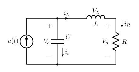
We can also derive a state space equation from physical laws. For example, consider the electrical circuit below,

Where $u(t)$ is the input and $V_0$ is the output.

Applying KCL gives us $i_c + i_L = u(t)$ .

Applying KVL gives us $V_L + V_0 - V_c = 0$ .

Applying element laws gives us $i_c = C \frac{d V_c}{dt}$ , $V_L = L \frac{di_L}{dt}$ , $V_0 = R i_R = R i_L$ .

Thus, we have the equations,

\begin{aligned} C \frac{d V_c}{dt} + i_L & = u \newline L \frac{d i_L}{dt} + R i_L + V_c & = 0. \end{aligned}

Let $x_1 = V_c$ and $x_2 = i_L$ , then we have the state equations,

\begin{aligned} \begin{bmatrix} \dot{x}_1 \newline \dot{x}_2 \end{bmatrix} & = \begin{bmatrix} 0 & -\frac{1}{C} \newline \frac{1}{L} & -\frac{R}{L} \end{bmatrix} \begin{bmatrix} x_1 \newline x_2 \end{bmatrix} + \begin{bmatrix} \frac{1}{C} \newline 0 \end{bmatrix} u \newline V_0 & = \begin{bmatrix} 0 & R \end{bmatrix} \begin{bmatrix} x_1 \newline x_2 \end{bmatrix}. \end{aligned}

However, as we have seen before, the solutions are not unique, if we instead write our systems of equations like this.

\begin{equation} \begin{aligned} C \frac{d V_c}{dt} + i_L & = u \newline \end{aligned} \end{equation}

\begin{equation} \begin{aligned} L \frac{d i_L}{dt} + R i_L + V_c & = 0. \end{aligned} \end{equation}

We can rewrite Equation (2) as,

\begin{aligned} V_c & = L \frac{di_L}{dt} + R i_L \newline \dot{V_c} & = L \frac{d^2 i_L}{dt^2} + R \frac{di_L}{dt} \newline \end{aligned}

Substitute this into Equation (1), we get,

\begin{aligned} C \frac{d V_c}{dt} + i_L & & = u \newline C \left( L \frac{d^2 i_L}{dt^2} + R \frac{di_L}{dt} \right) + i_L & = u \newline CL \frac{d^2 i_L}{dt^2} + CR \frac{di_L}{dt} + i_L & = u \newline \end{aligned}

Thus, our state variables are $x_1 = i_L$ and $x_2 = \frac{di_L}{dt}$ , and our state equations are,

\begin{aligned} \begin{bmatrix} \dot{x}_1 \newline \dot{x}_2 \end{bmatrix} & = \begin{bmatrix} 0 & 1 \newline -\frac{1}{CL} & -\frac{R}{L} \end{bmatrix} \begin{bmatrix} x_1 \newline x_2 \end{bmatrix} + \begin{bmatrix} 0 \newline \frac{1}{CL} \end{bmatrix} u \newline V_0 & = \begin{bmatrix} R & 0 \end{bmatrix} \begin{bmatrix} x_1 \newline x_2 \end{bmatrix}. \end{aligned}

Jacobian Linearization of Nonlinear Systems

Consider a nonlinear time-invariant system,

\begin{aligned} \dot{x} & = f(x, u) \quad x \in \mathbb{R}^n, u \in \mathbb{R}^m \newline y & = h(x, u) \quad y \in \mathbb{R}^p. \end{aligned}

Assume $f(0, 0) = 0$ and $h(0, 0) = 0$ , Let,

F = \frac{\partial f}{\partial x} \bigg|_{x = 0, u = 0} \in \mathbb{R}^{n \times n}

G = \frac{\partial f}{\partial u} \bigg|_{x = 0, u = 0} \in \mathbb{R}^{n \times m}

H = \frac{\partial h}{\partial x} \bigg|_{x = 0, u = 0} \in \mathbb{R}^{p \times n}

J = \frac{\partial h}{\partial u} \bigg|_{x = 0, u = 0} \in \mathbb{R}^{p \times m}

Then, by Taylor’s Theorem,

\begin{aligned} f(x, u) = Fx + Gu + \text{higher order terms} \newline h(x, u) = Hx + Ju + \text{higher order terms}. \end{aligned}

We call the system of equations,

\begin{aligned} \dot{x} & = Fx + Gu \newline y & = Hx + Ju \end{aligned}

as the (Jacobian) linerization of the above or small signal model.

Remark, for example, if the nonlinear functio is,

f(x, u) = \begin{bmatrix} f_1(x, u) \newline f_2(x, u) \end{bmatrix}

Then,

F = \begin{bmatrix} F_{11} & F_{12} \newline F_{21} & F_{22} \end{bmatrix} = \begin{bmatrix} \frac{\partial f_1}{\partial x_1} & \frac{\partial f_1}{\partial x_2} \newline \frac{\partial f_2}{\partial x_1} & \frac{\partial f_2}{\partial x_2} \end{bmatrix}

Similarly, we can get other matrices in the linear model.

Example 1 (Pendulum)

Consider the pendulum system we have seen before, the equation of motion is,

\ddot{\theta} + \frac{g}{l} \sin(\theta) = \frac{T_c}{ml^2}

Let’s denote $\omega = \sqrt{\frac{g}{l}}$ and $u = \frac{T_c}{ml^2}$ .

The state-variable form with $x = \begin{bmatrix} x_1 & x_2 \end{bmatrix}^T = \begin{bmatrix} \theta & \dot{\theta} \end{bmatrix}^T$ is,

\dot{x} = \begin{bmatrix} \dot{x}_1 \newline \dot{x}_2 \end{bmatrix} = \begin{bmatrix} x_2 \newline -\omega^2 \sin(x_1) + u \end{bmatrix} = f(x, u)

We can linearize this system by finding the Jacobian matrices.

The partial derivatives evaluated at $x = 0$ and $u = 0$ are,

\begin{aligned} \frac{\partial f_1}{\partial x_1} & = 0 \newline \frac{\partial f_1}{\partial x_2} & = 1 \newline \frac{\partial f_2}{\partial x_1} & = -\omega^2 \newline \frac{\partial f_2}{\partial x_2} & = 0 \newline \frac{\partial f_1}{\partial u} & = 0 \newline \frac{\partial f_2}{\partial u} & = 0. \end{aligned}

Thus, the Jacobian matrices are,

F = \begin{bmatrix} 0 & 1 \newline -\omega^2 & 0 \end{bmatrix}

G = \begin{bmatrix} 0 \newline 1 \end{bmatrix}

H = \begin{bmatrix} 0 & 0 \end{bmatrix}

J = \begin{bmatrix} 0 \end{bmatrix}

Thus, the linearized system is,

\dot{x} = \begin{bmatrix} 0 & 1 \newline -\omega^2 & 0 \end{bmatrix} x + \begin{bmatrix} 0 \newline 1 \end{bmatrix} u

Remark 1

The state of a system at time $t_0$ is a set of variables at $t_0$ that together with input functions determines uniquely the behavior of the system for all $t \geq t_0$ .

A system can have different states and the states do not have to have physical meaning.

Solution of State Space Equation

The solution of the state space equation that satifies an initial condition can be a bit tricky.

Given $\dot{x}(t) = Fx(t) + Gu(t) \quad t \geq t_0, x \in \mathbb{R}^n, u \in \mathbb{R}^m$ and $x_0, u(t), t \geq t_0$ are given.

Find $x(t), t \leq t_0$ subject to $x(t_0) = x_0$ and $x(t)$ satisfies the above.

Here $x_0$ is called the initial condition and $u(t)$ is called the input.

The solution is,

x(t) = e^{F(t - t_0)} \left[ x_0 + \int_{t_0}^{t} e^{-F \tau} G u(\tau) d\tau \right].

Special Case: $n=m=1$

Given $\dot{x}(t) = Fx(t) + Gu(t) \quad t \geq t_0, x \in \mathbb{R}^n, u \in \mathbb{R}^m$ and $x_0, u(t), t \geq t_0$ are given.

Since $e^{Ft}(e^{-Ft} x(t))^{\prime} = -Fx(t) + \dot{x}(t)$ , the above implies,

\begin{aligned} e^{Ft}(e^{-Ft} x(t))^{\prime} & = e^{-Ft} G u(t) \newline e^{-Ft} x(t) - e^{-Ft_0} x(t_0) & = \int_{t_0}^{t} e^{-F \tau} G u(\tau) d\tau \newline x(t) & = e^{F(t - t_0)} x_0 + \int_{t_0}^{t} e^{F(t - \tau)} G u(\tau) d\tau \newline & = e^{F(t - t_0)} \left[ x_0 + \int_{t_0}^{t} e^{-F \tau} G u(\tau) d\tau \right]. \end{aligned}

Transfer Function of SISO Systems

Consider the SISO system,

\begin{aligned} \dot{x}(t) & = Fx(t) + Gu(t) \newline y(t) & = Hx(t) + Ju(t). \end{aligned}

where $u \in \mathbb{R}, y \in \mathbb{R}, x \in \mathbb{R}^n, F \in \mathbb{R}^{n \times n}, G \in \mathbb{R}^{n \times 1}, H \in \mathbb{R}^{1 \times n}, J \in \mathbb{R}$ .

The transfer function of the system is defined as,

P(s) = \frac{Y(s)}{U(s)} \bigg|_{x(0) = 0}.

Performing Laplace Transform on the state equations gives,

\begin{aligned} sX(s) - x_0 & = FX(s) + GU(s) \newline Y(s) & = HX(s) + JU(s). \end{aligned}

Thus,

\begin{aligned} X(s) & = (sI - F)^{-1} GU(s) + (sI - F)^{-1} x_0 \newline Y(s) & = H(sI - F)^{-1} GU(s) + (H(sI - F)^{-1} x_0 + JU(s)). \end{aligned}

The transfer function is then,

P(s) = \frac{Y(s)}{U(s)} = H(sI - F)^{-1} G + J.

Remarks

$P(s) = H(sI - F)^{-1} G + J = \frac{\beta(s)}{\alpha(s)}$ is a rational function.

where $\alpha(s)$ is the characteristic polynomial of $F$ with degree $n$ , $\beta{s}$ is polynomial of degree $n$ when $J \neq 0$ or degree $< n$ when $J = 0$ .

$P(s)$ is a proper rational if degree of $\beta(s) \leq$ degree of $\alpha(s)$ .
$P(s)$ is a strictly proper rational function when $J = 0$ , i.e., degree of $\beta(s) <$ degree of $\alpha(s)$ .

In general, we can write,

P(s) = \frac{b_{n - m} s^m + b_{n - m - 1} s^{m - 1} + \ldots + b_n}{s^n + a_1 s^{n - 1} + \ldots + a_n}.

where $b_{n - m} \neq 0$ and $0 \leq m \leq n$ and the integer $(n - m)$ is called the relative degree of the system.

$P(s) = H(sI - F)^{-1} G + J = \frac{\det \begin{bmatrix} sI - F & -G \newline H & J \end{bmatrix}}{\det(sI - F)}$ .

The eigenvalues of $F$ are called natural frequency or natural mode of the system.

Let,

P(s) = \frac{\beta(s)}{\alpha(s)} = \frac{\gamma(s) \beta_d(s)}{\gamma(s) \alpha_d(s)} = \frac{\beta_d(s)}{\alpha_d(s)},

where $\gamma(s)$ is the greatest common divisor of $\beta(s)$ and $\alpha(s)$ . Thus, $\beta_d(s)$ and $\alpha_d(s)$ are coprime (the greatest common divisor of them is a constant).

The roots of $\alpha_d(s)$ are called the poles of $P(s)$ and the roots of $\beta_d(s)$ are called the zeros of $P(s)$ .

All poles of $P(s)$ are the eigenvalues of $F$ , but some eigenvalues of $F$ may not be the poles of $P(s)$ !