Part 7 - State Space Realization

State Space Realization

The problem of deriving a linear state space equation from a higher ODE or transfer function is called realization.

we have seen some realization examples from ODEs to the state space equation, we also introduced how to get a transfer function from the state space function.

But now, if we have a transfer function, what is the state space equation?

Given,

P(s) = \frac{\beta(s)}{\alpha(s)} = \frac{b_0s^n + b_1s^{n - 1} + \ldots + b_{n - 1} s + b_n}{s^n + a_1 s^{n - 1} + \ldots + a_{n - 1} s + a_n}

We want to find $\hat{n} \geq n, F \in \mathbb{R}^{\hat{n} \times \hat{n}}, G \in \mathbb{R}^{\hat{n} \times 1}, H \in \mathbb{R}^{1 \times \hat{n}}$ and $J \in \mathbb{R}$ such that,

P(s) = H(sI - F)^{-1}G + J

We call the system,

\begin{aligned} \dot{x} &= Fx + Gu \newline y &= Hx + Ju \end{aligned}

a state space realization of $P(s)$ or $(F, G, H, J)$ a realization. $\hat{n}$ is the dimension of the realization.

From Transfer Function to State Space

Consider the following system which has a simple transfer function,

P(s) = \frac{s + 2}{s^2 + 7s + 12}

Let $F = \begin{bmatrix} -7 & -12 \newline 1 & 0 \end{bmatrix}, G = \begin{bmatrix} 1 \newline 0 \end{bmatrix}, H = \begin{bmatrix} 1 & 2 \end{bmatrix}$ and $J = 0$ .

Therefore,

\begin{aligned} \begin{bmatrix} \dot{x}_1 \newline \dot{x}_2 \end{bmatrix} &= \begin{bmatrix} -7 & -12 \newline 1 & 0 \end{bmatrix} \begin{bmatrix} x_1 \newline x_2 \end{bmatrix} + \begin{bmatrix} 1 \newline 0 \end{bmatrix} u \newline y &= \begin{bmatrix} 1 & 2 \end{bmatrix} \begin{bmatrix} x_1 \newline x_2 \end{bmatrix} \end{aligned}

This is a realization of the transfer function $P(s)$ .

If we observe the solution and our original transfer function, we can see a pattern.

Control Canonical Form Realization

Let,

F = \begin{bmatrix} -a_1 & -a_2 & \ldots & -a_{n - 1} & -a_n \newline 1 & 0 & \ldots & 0 & 0 \newline 0 & 1 & \ldots & 0 & 0 \newline \vdots & \vdots & \ddots & \vdots & \vdots \newline 0 & 0 & \ldots & 1 & 0 \end{bmatrix} \triangleq A_c

G = \begin{bmatrix} 1 \newline 0 \newline \vdots \newline 0 \end{bmatrix} \triangleq B_c, H = \begin{bmatrix} b_1 & b_2 & \ldots & b_{n} \end{bmatrix} \triangleq C_c, J = 0 \triangleq D_c

C_c(sI - A_c)^{-1}B_c = \frac{b_1s^{n - 1} + b_2s^{n - 2} + \ldots + b_n}{s^n + a_1s^{n - 1} + \ldots + a_n}

Companion Matrix

The matrix $A_c$ is determined by the coefficients of the polynomial $\alpha(s)$ and is called the companion matrix of $\alpha(s)$ .

We have a nice property of the companion matrix,

Proposition 1

$\det(sI - A_c) = \alpha(s) = s^n + a_1s^{n - 1} + \ldots + a_n$

Proof

For $n = 3$ :

A_c = \begin{bmatrix} -a_1 & -a_2 & -a_3 \newline 1 & 0 & 0 \newline 0 & 1 & 0 \end{bmatrix} \implies sI - A_c = \begin{bmatrix} s + a_1 & a_2 & a_3 \newline -1 & s & 0 \newline 0 & -1 & s \end{bmatrix}

Thus,

\begin{aligned} \det(sI - A_c) & = -(-1) \begin{vmatrix} s + a_1 & a_3 \newline -1 & 0 \end{vmatrix} + s \begin{vmatrix} s + a_1 & a_2 \newline -1 & s \end{vmatrix} \newline & = a_3 + s((s + a_1)s + a_2) \newline & = s^3 + a_1s^2 + a_2s + a_3 \end{aligned}

Observer Canonical Form Realization

Let,

A_o = A_c^T = \begin{bmatrix} -a_1 \newline \vdots & I_{n - 1} \newline -a_{n - 1} \newline -a_n & \mathbf{0}_{1 \times (n - 1)} \end{bmatrix}

B_o = C_c^T = \begin{bmatrix} b_1 \newline \vdots \newline b_n \end{bmatrix}, C_o = B_c^T = \begin{bmatrix} 1 & 0 & \ldots & 0 \end{bmatrix}, D_o = 0

Then,

C_o(sI - A_o)^{-1}B_o = P(s) = \frac{b_1s^{n - 1} + b_2s^{n - 2} + \ldots + b_n}{s^n + a_1s^{n - 1} + \ldots + a_n}

I.e.,

\begin{aligned} \dot{x} &= A_o x + B_o u \newline y &= C_o x + D_o u \end{aligned}

is also a realization of $P(s)$ .

Example 1

Let,

P(s) = \frac{b_1 s^2 + b_2 s + b_3}{s^3 + a_1 s^2 + a_2 s + a_3}

Find the control canonical form realization and observer canonical form realization.

Let’s start with control canonical form realization,

A_c = \begin{bmatrix} -a_1 & -a_2 & -a_3 \newline 1 & 0 & 0 \newline 0 & 1 & 0 \end{bmatrix}

B_c = \begin{bmatrix} 1 \newline 0 \newline 0 \end{bmatrix}

C_c = \begin{bmatrix} b_1 & b_2 & b_3 \end{bmatrix}

For observer canonical form realization,

A_o = A_c^T = \begin{bmatrix} -a_1 & 1 & 0 \newline -a_2 & 0 & 1 \newline -a_3 & 0 & 0 \end{bmatrix}

B_o = C_c^T = \begin{bmatrix} b_1 \newline b_2 \newline b_3 \end{bmatrix}

C_o = B_c^T = \begin{bmatrix} 1 & 0 & 0 \end{bmatrix}

Remark 1

Nonuniquess of realization, as we have seen previously, the realizations are not unique (we will discuss this shortly).
The dimension of a realization can be any integer greater or equal to $n$ . If $\alpha(s)$ and $\beta(s)$ are coprime, then the minimal dimension of a realization of a transfer function is equal to n.
The transfer function of a state equation is invariant under a state transformation.

What is a Good Realization?

A realization can be viewed as a modeling method of physical system.

Since realizations are not unique, they can be good and bad realizations.

From the control point of view, we need to determine what makes a good realization.

Controllability and observability are two criterions to determine a good realization.

Controllability Matrix & Observability Matrix

The matrix,

\begin{bmatrix} B_c & A_cB_c & \ldots & A_c^{n - 1}B_c \end{bmatrix}

is called the controllability matrix of the system.

The matrix,

\begin{bmatrix} C_o \newline C_oA_o \newline \vdots \newline C_oA_o^{n - 1} \end{bmatrix}

is called the observability matrix of the system.

NB: The elements of these matrices are matrices, for example,

Let $A = \begin{bmatrix} 1 & 2 \newline 3 & 4 \end{bmatrix}$ and $B = \begin{bmatrix} 5 & 6 \newline 7 & 8 \end{bmatrix}$ , then the matrix $[A B]$ is,

\begin{bmatrix} 1 & 2 & 5 & 6 \newline 3 & 4 & 7 & 8 \end{bmatrix}

We are not going into the formal proof, but it can be verified that,

\text{rank} \begin{bmatrix} B_c & A_cB_c & \ldots & A_c^{n - 1}B_c \end{bmatrix} = n

and

\text{rank} \begin{bmatrix} C_o \newline C_oA_o \newline \vdots \newline C_oA_o^{n - 1} \end{bmatrix} = n

Remark

One can always transform a given state description to control canonical form if and only if the controllability matrix is nonsingular (i.e., full rank).

Controllability

From the name, it suggests that, to what extent can the input $u$ affect the state $x$ .

Let’s go with this intuition for a moment.

Let’s say we have two state variables $x_1$ and $x_2$ .

The system is described by the following equations,

\begin{aligned} \dot{x_1} & = x_1, x_1(0) x_{10} \newline \dot{x_2} & = x_2 + u, x_2(0) = x_{20} \end{aligned}

Thus, $x_1$ and $x_2$ in the time domain are,

\begin{aligned} x_1(t) & = e^t x_{10} \newline x_2(t) & = e^t x_{20} + e^t \int_0^t e^{-\tau} u(\tau) d\tau \end{aligned}

No matter how $u(t)$ is chosen or designed, it cannot affect $x_1(t)$ .

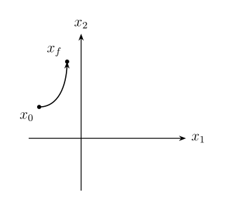
Note, this doesn’t mean we can specifically design a system as a whole to go from a starting point $x_0$ to a final point $x_f$ given the right conditions.

But since this generally doesn’t, hold, meaning we can not go from an arbitrary starting point to an arbitrary final point, we say the system is uncontrollable.

Let’s now properly define controllability.

Definition 1 (Controllability)

The LTI system,

\dot{x} = Fx + Gu, x(0) = 0, t \geq 0

where $F \in \mathbb{R}^{n \times n}$ and $G \in \mathbb{R}^{n \times 1}$ is controllable on $[0, t_f]$ for some $t_f > 0$ , if given any initial state $x_0$ and final state $x_f$ , there exists a pieacewise continuous input $u(t)$ subject to the solutuion of the system, satifies

x(t_f) = x_f

Remark 2

It will be seen later that whether a system is controllable depends on $F$ and $G$ , we also say that the pair $\{F, G\}$ is controllable or uncontrollable.

Theorem 1 (Criterion for Controllability)

The system is controllable if and only if,

\text{rank} \begin{bmatrix} G & FG & \ldots & F^{n - 1}G \end{bmatrix} = n

Example 2

Let’s consider the system,

F = \begin{bmatrix} 0 & 1 \newline -2 & -1 \end{bmatrix}, G = \begin{bmatrix} 0 \newline 1 \end{bmatrix}

We can see that this system is of order two, so let’s first calculate $FG$ .

FG = \begin{bmatrix} 1 \newline -1 \end{bmatrix}

Thus, the controllability matrix is,

\begin{bmatrix} 0 & 1 \newline 1 & -1 \end{bmatrix}

For matrices of size $2 \times 2$ , we can easily calculate the determinant,

\det \begin{bmatrix} 0 & 1 \newline 1 & -1 \end{bmatrix} = (0 \cdot -1) - (1 \cdot 1) = -1

Since the determinant is not zero, the controllability matrix is full rank, and the system is controllable.

On the other hamd, if

F = \begin{bmatrix} 1 & 0 \newline 0 & 1 \end{bmatrix}, G = \begin{bmatrix} 0 \newline 1 \end{bmatrix}

FG = \begin{bmatrix} 0 \newline 1 \end{bmatrix}

Then, the controllability matrix is,

\begin{bmatrix} 0 & 0 \newline 1 & 1 \end{bmatrix}

The determinant of this matrix is zero, so the system is uncontrollable.

Recall (Rank of a matrix)

(This is just a refresher, skip if you are already familiar with this)

Let $A = [a_{ij}]$ be a $n \times m$ matrix. If $n = m$ , then $A$ has full rank if and only if $A$ is nonsingular if and only if $\det(A) \neq 0$ .

If $n < m$ , then A has full rank if and only if $A$ contains a nonsingular $n \times n$ submatrix. An $n \times n$ submatrix of $A$ can be obtained from $A$ by removing any $m - n$ columns of $A$ .

If $n > m$ then $A$ has full rank if and only if $A$ contains a nonsingular $m \times m$ submatrix. An $m \times m$ submatrix of $A$ can be obtained from $A$ by removing any $n - m$ rows of $A$ .

Observability

Observability is the dual of controllability. It is the extent to which the state $x$ can be determined from the output $y$ .

The state $x$ may not have any physical meaning and may not be measurable. It is desirable to be able to estimate $x(t)$ from the information of $y(t)$ and $u(t)$ .

If this is indeed the case, the state $x(t)$ is said to be observable from the input and output.

Definition 2 (Observability)

The LTI system,

\begin{aligned} \dot{x} & = Fx + Gu \quad x(0) = x_0 \newline y & = Hx + Ju \quad t \geq 0 \end{aligned}

is observable if for any $t > 0$ , $x(t)$ can be determined from $y(t)$ and $u(t)$ .

Theorem 2 (Criterion for Observability)

The system is observable if and only if,

\text{rank} \begin{bmatrix} H \newline HF \newline \vdots \newline HF^{n - 1} \end{bmatrix} = n

Example 3

Let’s consider the system,

F = \begin{bmatrix} 0 & 0 & 2 \newline 0 & 0 & 1 \newline -2 & 0 & 0 \end{bmatrix}, G = \begin{bmatrix} 1 & 0 \newline 0 & 0 \newline 0 & 1 \end{bmatrix}, H = \begin{bmatrix} 1 & 0 & 0 0 & 0 & 1 \end{bmatrix}

We can see that this system is of order three, so let’s first calculate $F^2$ , $HF$ , and $HF^2$ .

F^2 = \begin{bmatrix} -4 & 0 & 0 \newline -2 & 0 & 0 \newline 0 & 0 & -2 \end{bmatrix}

HF = \begin{bmatrix} 0 & 0 & 2 \newline -2 & 0 & 0 \end{bmatrix}

HF^2 = \begin{bmatrix} -4 & 0 & 0 \newline 0 & 0 & -2 \end{bmatrix}

Thus, the observability matrix is,

\begin{bmatrix} 1 & 0 & 0 \newline 0 & 0 & 1 \newline 0 & 0 & 2 \newline -2 & 0 & 0 \newline -4 & 0 & 0 \newline 0 & 0 & -2 \end{bmatrix}

We can see that we have a zero column in the matrix, which means the columns are not linearly independent which means not full rank, so the system is not observable.

Example 4

Let’s consider the system,

F = \begin{bmatrix} 0 & -0.1 \newline 1 & -0.2 \end{bmatrix}, H = \begin{bmatrix} 0 & 1 \end{bmatrix}

We can see that this system is of order two, so let’s first calculate $HF$ .

HF = \begin{bmatrix} 1 & -0.2 \end{bmatrix}

Thus, the observability matrix is,

\begin{bmatrix} 0 & 1 \newline 1 & -0.2 \end{bmatrix}

Which we can see has a non-zero determinant, so the system is observable.

Properties and Remarks

$\{A_c, B_c, C_c\}$ is always controllable, but may not be observable. But if $C_c(sI - A_c)^{-1} B_c$ is irreducible, then $\{A_c, B_c, C_c\}$ is also observable.
$\{A_o, B_o, C_o\}$ is always observable, but may not be controllable. But if $C_o(sI - A_o)^{-1} B_o$ is irreducible, then $\{A_o, B_o, C_o\}$ is also controllable.
Define $C(F, G) = \begin{bmatrix} G & FG & \ldots & F^{n - 1}G \end{bmatrix}$ and call it the controllability matrix, and $O(H, F) = \begin{bmatrix} H \newline HF \newline \vdots \newline HF^{n - 1} \end{bmatrix}$ and call it the observability matrix.