Part 4 - Simple Linear Regression

Introduction

The main objective of many statistical investigations is to make predictions.

For instance, an engineer may wish to predict the amount of oxide that will form on the surface of a metal baked in an oven for one hour at 200$^{\circ}$C, or the amount of deformation of a ring subjected to a certain compressive force.

Usually, such predictions require a formula which relates the dependent variable whose value we want to predict (or called response) to one or more other variables, usually called predictors (or regressors).

The collection of statistical tools for this is called regression analysis.

Simple Linear Regression

The simplest form of regression analysis is simple linear regression, which involves a single predictor and a single response variable.

where:

• $Y$ is the response variable.
• $X$ is the predictor variable.
• $\beta_0$ is the intercept.
• $\beta_1$ is the slope.

Assume that $\mathbb{E}(e) = 0$ and $\text{Var}(e) = \sigma^2$.

Suppose we fix $X = x$, meaning

with mean $\mathbb{E}(Y) = \beta_0 + \beta_1 x$ and variance $\text{Var}(Y) = \sigma^2$ ($Y$ is normal if $e$ is normal).

The linear function $\beta_0 + \beta_1 x$ is thus the function giving the mean value of $Y$ for each possible value of $X$.

It is called the regression function (or regression line) and will be denoted as,

The slope $\beta_1$ is the change in mean of $Y$ for one unit change in $X$, the intercept $\beta_0$ is the mean value of $Y$ when $X = 0$.

Least Squares Estimator

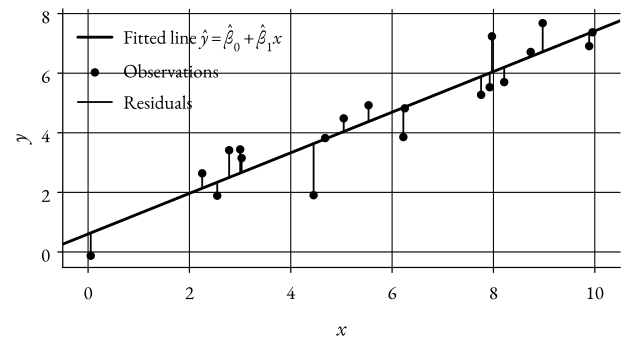
Gauss proposed estimating $\beta_0$ and $\beta_1$ to minimize the sum of the squares of the vertical deviations between the observed responses and the fitted line.

These deviations are called the residuals.

For any “candidate” straight line $Y = a + bX$, we can write $R(a, b) = \sum_{i = 1}^N (Y_i - (a + bX_i))^2$.

The minimizers are $(\hat{\beta_0}, \hat{\beta_1})$, with

and

where $\bar{X} = \frac{1}{n} \sum_i X_i$ and $\bar{Y} = \frac{1}{n} \sum_i Y_i$.

We can clean up this by defining the following quantities:

Thus, we have,

and

The variance $\sigma^2$ of the error term $e = Y - (\beta_0 + \beta_1 X)$ is another unknown parameter.

The residuals,

can be regarded as a ‘sample’

First, it can be checked that,

(by definition of the estimated coefficient $\hat{\beta}_0$ and $\hat{\beta}_1$).

Therefore, an unbiased estimate of $\sigma^2$ is,

Inferences

From now on we will assume that the value of the predictors are deterministic (or we condition on X).

We note that $Y_i | (X_i = x_i) \sim N(\beta_0 + \beta_1 x_i, \sigma^2)$.

Then, because $\sum_i (x_i - \bar{x}) = 0$, we can write,

The sampling distribution of $\hat{\beta_1}$ is normal with mean $\beta_1$ and variance $\sigma^2 / s_{xx}$.

Now we can write,

which is again a linear combination of normal random variables (the $Y_i$’s and $\hat{\beta}_1$).

Thus, the estimator of $\beta_0$ is also normally distributed.

The sampling distribution of $\hat{\beta_0}$ is normal with mean $\beta_0$ and variance $\sigma^2 \left(\frac{1}{n} + \frac{\bar{x}^2}{s_{xx}}\right)$.

Confidence Interval

If we have the hypothesis,

We have $\sqrt{s_{xx}} \frac{\hat{\beta}_1 - \beta_1}{\sigma} \sim N(0, 1)$.

Replacing $\sigma$ with its estimator $S$, we find,

The rejection region is then,

The $p$-value is,

where $t_0 = \frac{\hat{\beta_1}}{s / \sqrt{s_{xx}}}$ and $T$ is a random variable with distribution $t_{n - 2}$.

So, the CI for $\beta_1$ is,

Confidence Interval on the Mean Response

For a specified value of $X$, say, $x$, we want a confidence interval for,

we have an estimator,

and

Replacing the unkown $\sigma$ by its estimator $S$, we get,

and the CI is,

Prediction of new observations

An important application is predicting new or future observations $Y$ corresponding to a specified level $X = x$.

This is different to estimating the mean response.

$\mu_{Y | X = x}$ at $X = x$, a predicted value is $\hat{y}(x) = \beta_0 + \beta_1 x$.

We can derive,

which leads to the following prediction interval,

Remarks

1. A prediction interval for $Y$ at $X = x$ will always be longer than the CI for $\mu_{Y | X = x}$ because there is much more variability in one observation than in an average.

2. As $n$ gets larger ($n \to \infty$), the width of CI for $\mu_{Y | X = x}$ decreases to 0, buy this is not the case for the prediction interval.

Analysis of Variance (ANOVA)

The most interesting test for simple linear regression is probably,

We previously used $t$-test,

There is an alternative (and equivalent) test, the $F$-test based on analysis of variance.

Firstly, let’s define some quantities,

where $SST$ is the total sum of squares, $SS_{\text{reg}}$ is the regression sum of squares, and $RSS$ is the residual sum of squares.

For the $F$-test, we use,

We reject $H_0$ if $F > F_{1 - \alpha, 1, n - 2}$.

Analysis of Variance Table

The ANOVA table is a table that shows the sources of variation in an experiment.

1
changeover_times<-read.table("changeover_times.txt", header=TRUE)
2
attach(changeover_times)
3

4
m1<-lm(Changeover~New)
5
summary(m1)
6

7
par(mfrow=c(2,2))
8
plot(New,Changeover,xlab="Dummy variable, New",ylab="Change Over Time")
9
abline(lsfit(New,Changeover))
10
boxplot(Changeover~New,xlab="Dummy variable, New",ylab="Change Over Time")
11
boxplot(Changeover~Method,ylab="Change Over Time",xlab="Method")
12

13
# p-value
14
pval<-2*pt(-2.254,df=118)
15
pval
16

17
# equivalently, using two sample test
18
t.test(Changeover[New==0],Changeover[New==1],var.equal = TRUE)
19
t.test(Changeover[New==0],Changeover[New==1],var.equal = FALSE)
20

21
detach(changeover_times)

1
leverage<-hatvalues(m1)
2
# or influence(m1)$hat
3

4
stdres<-rstandard(m1)
5
res<-m1$residuals
6
# or residuals(m1)