Introduction
Most SDEs take the form,
d x ( t ) = f ( x ( t ) , t ) d t ⏟ drift + L ( x ( t ) , t ) d β ( t ) ⏟ diffusion , \begin{equation}
dx(t) = \underbrace{f(x(t), t) \, dt}_{\text{drift}} + \underbrace{L(x(t), t) \, d\beta(t)}_{\text{diffusion}},
\end{equation} d x ( t ) = drift f ( x ( t ) , t ) d t + diffusion L ( x ( t ) , t ) d β ( t ) , where x ( t ) x(t) x ( t ) β ( t ) \beta(t) β ( t ) 1
The SDE in Equation (1) is shorthand for the (Itô, teaser!) integral equation,
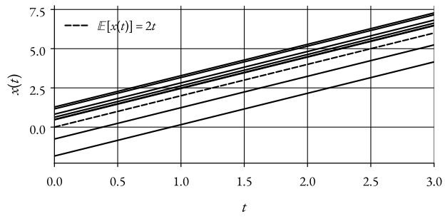
x ( t ) − x ( t 0 ) = ∫ t 0 t f ( x ( s ) , s ) d s + ∫ t 0 t L ( x ( s ) , s ) d β ( s ) . x(t) - x(t_0) = \int_{t_0}^{t} f(x(s), s) \, ds + \int_{t_0}^{t} L(x(s), s) \, d\beta(s). x ( t ) − x ( t 0 ) = ∫ t 0 t f ( x ( s ) , s ) d s + ∫ t 0 t L ( x ( s ) , s ) d β ( s ) . Figure 1: SDE with only drift (an ODE)Suppose f ( x , t ) = 2 , L ( x , t ) = 0 f(x, t) = 2, L(x, t) = 0 f ( x , t ) = 2 , L ( x , t ) = 0 ⇒ d x d t = 2 \Rightarrow \frac{dx}{dt} = 2 ⇒ d t d x = 2
We also assume that x ( 0 ) ∼ N ( 0 , 2 ) x(0) \sim \mathcal{N}(0, 2) x ( 0 ) ∼ N ( 0 , 2 ) Figure 1 .
Definition 1 (Definition: Brownian motion – β ( t ) \beta(t) β ( t )
Any increment Δ β = β ( t ′ ) − β ( t ) ∼ N ( 0 , ( t ′ − t ) Q ) . \Delta \beta = \beta(t^{\prime}) - \beta(t) \sim \mathcal{N}(0, (t^{\prime} - t) Q). Δ β = β ( t ′ ) − β ( t ) ∼ N ( 0 , ( t ′ − t ) Q ) . Q = 1 Q = 1 Q = 1
Increments are independent unless intervals overlap.
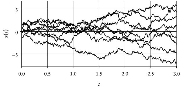
β ( 0 ) = 0 \beta(0) = 0 β ( 0 ) = 0 Figure 2: SDE with only diffusion.Suppose f ( x , t ) = 0 , L ( x , t ) = 2 f(x, t) = 0, L(x, t) = 2 f ( x , t ) = 0 , L ( x , t ) = 2 ⇒ d x ( t ) = 2 d β ( t ) \Rightarrow dx(t) = 2 \, d\beta(t) ⇒ d x ( t ) = 2 d β ( t )
We also assume that x ( 0 ) ∼ N ( 0 , 1 ) x(0) \sim \mathcal{N}(0, 1) x ( 0 ) ∼ N ( 0 , 1 ) Figure 2 .
To sample x ( t ) x(t) x ( t ) x ( 0 ) ∼ p ( x ( 0 ) ) x(0) \sim p(x(0)) x ( 0 ) ∼ p ( x ( 0 ))
x ( t + Δ t ) = x ( t ) + f ( x ( t ) , t ) Δ t + L ( x ( t ) , t ) z , z ∼ N ( 0 , Δ t ) . \begin{equation}
x(t + \Delta t) = x(t) + f(x(t), t) \Delta t + L(x(t), t)z, \quad z \sim \mathcal{N}(0, \Delta t).
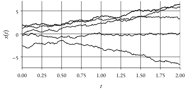
\end{equation} x ( t + Δ t ) = x ( t ) + f ( x ( t ) , t ) Δ t + L ( x ( t ) , t ) z , z ∼ N ( 0 , Δ t ) . Figure 3: Sample of a SDE.We can use Equation (2) to sample from,
d x ( t ) = 0.5 x d t + d β ( t ) , d x(t) = 0.5x \, dt + d \beta(t), d x ( t ) = 0.5 x d t + d β ( t ) , which corresponds to f ( x , t ) = 0.5 x f(x, t) = 0.5x f ( x , t ) = 0.5 x L ( x , t ) = 1 L(x, t) = 1 L ( x , t ) = 1 Figure 3 .
Motivation and Dynamic Models
SDEs are commonly used to model object dynamics (cars, airplanes, etc).
Often, time-discretized versions are used for filtering, smoothing, and prediction.
Constant Velocity Models (Scalar Example)
Suppose x ( t ) = [ x ( t ) v ( t ) ] T \mathbf{x}(t) = \begin{bmatrix} x(t) & v(t) \end{bmatrix}^T x ( t ) = [ x ( t ) v ( t ) ] T
According to the constant velocity model,
d x ( t ) = [ 0 1 0 0 ] x ( t ) d t + [ 0 q ] d β ( t ) , ⇔ = [ v ( t ) d t 0 ] + [ 0 q d β ( t ) ] . \begin{align*}
d \mathbf{x}(t) & =
\begin{bmatrix}
0 & 1 \newline
0 & 0
\end{bmatrix} \mathbf{x}(t) \, dt +
\begin{bmatrix}
0 \newline
q
\end{bmatrix} d \beta(t), \newline
\Leftrightarrow & =
\begin{bmatrix}
v(t) \, dt \newline
0
\end{bmatrix} +
\begin{bmatrix}
0 \newline
q \, d\beta(t)
\end{bmatrix}.
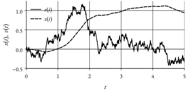
\end{align*} d x ( t ) ⇔ = [ 0 0 1 0 ] x ( t ) d t + [ 0 q ] d β ( t ) , = [ v ( t ) d t 0 ] + [ 0 q d β ( t ) ] . The position follows the velocity, whereas the velocity is a Brownian motion.
Figure 4: Constant Velocity Model with x ( 0 ) = v ( 0 ) = 0 x(0) = v(0) = 0 x ( 0 ) = v ( 0 ) = 0 The Ornstein-Uhlenbeck process 2
d v ( t ) = − θ v ( t ) d t + σ d β ( t ) , dv(t) = -\theta v(t) \, dt + \sigma \, d\beta(t), d v ( t ) = − θ v ( t ) d t + σ d β ( t ) , is used in several fields, e.g., in physics to model particles moving with friction.
The Black-Scholes equation 3
A basic version of this equation is,
d s ( t ) = μ s ( t ) d t + σ s ( t ) d β ( t ) , ds(t) = \mu s(t) \, dt + \sigma s(t) \, d\beta(t), d s ( t ) = μ s ( t ) d t + σ s ( t ) d β ( t ) , where s ( t ) s(t) s ( t )
The stochastic Lotka-Volterra 4
d x ( t ) = x ( t ) ( a − b y ( t ) ) d t + σ 1 x ( t ) d β 1 ( t ) , d y ( t ) = y ( t ) ( − c + d x ( t ) ) d t + σ 2 y ( t ) d β 2 ( t ) . \begin{align*}
dx(t) & = x(t)(a - b y(t)) \, dt + \sigma_1 x(t) \, d\beta_1(t), \newline
dy(t) & = y(t)(-c + d x(t)) \, dt + \sigma_2 y(t) \, d\beta_2(t).
\end{align*} d x ( t ) d y ( t ) = x ( t ) ( a − b y ( t )) d t + σ 1 x ( t ) d β 1 ( t ) , = y ( t ) ( − c + d x ( t )) d t + σ 2 y ( t ) d β 2 ( t ) . Here, x ( t ) x(t) x ( t ) y ( t ) y(t) y ( t ) β 1 ( t ) \beta_1(t) β 1 ( t ) β 2 ( t ) \beta_2(t) β 2 ( t )
Diffusion can be used as a (deep) generative model as well (and this is what we are mostly interested in).
The basic idea is,
Recursively remove structure from data (make it noisier!).
Train network to remove noise and obtain structure again .
Generate (new) data by feeding noise to the trained network.
The forward process is generally an SDE,
d x ( t ) = f ( x , t ) d t + L ( t ) d β ( t ) . d x(t) = f(x, t) \, dt + L(t) \, d\beta(t). d x ( t ) = f ( x , t ) d t + L ( t ) d β ( t ) . We are going to get a solid understanding of theoretical results used to train and perform inference in these models.
Image generation is arguably the most well-known application. A few other examples are,
Besides bridging noise and data distributions we can bridge, e.g., low- and high-resolution images.
Molecular and drug design, e.g., protein structures.
Sequential data, e.g., human pose sequences and financial data.
Motion planning and reinforcement learning with diffusion policies.
The Engineering Approach: White Noise
Recall that we study SDEs on the form,
d x ( t ) = f ( x ( t ) , t ) d t + L ( x ( t ) , t ) d β ( t ) , x ( t ) − x ( t 0 ) = ∫ t 0 t f ( x ( s ) , s ) d s + ∫ t 0 t L ( x ( s ) , s ) d β ( s ) . \begin{align*}
dx(t) & = f(x(t), t) \, dt + L(x(t), t) \, d\beta(t), \newline
x(t) - x(t_0) & = \int_{t_0}^t f(x(s), s) \, ds + \int_{t_0}^t L(x(s), s) \, d\beta(s).
\end{align*} d x ( t ) x ( t ) − x ( t 0 ) = f ( x ( t ) , t ) d t + L ( x ( t ) , t ) d β ( t ) , = ∫ t 0 t f ( x ( s ) , s ) d s + ∫ t 0 t L ( x ( s ) , s ) d β ( s ) . In engineering literature, the notation d β ( t ) d \beta(t) d β ( t )
Imagine for a second that if β ( t ) \beta(t) β ( t ) w ( t ) = d β ( t ) d t w(t) = \frac{d \beta(t)}{dt} w ( t ) = d t d β ( t )
d x ( t ) d t = f ( x , t ) + L ( x , t ) w ( t ) , x ( t 1 ) − x ( t 0 ) = ∫ t 0 t 1 f ( x ( s ) , s ) d s + ∫ t 0 t 1 L ( x ( s ) , s ) w ( s ) d s , \begin{align*}
\frac{dx(t)}{dt} & = f(x, t) + L(x, t) w(t), \newline
x(t_1) - x(t_0) & = \int_{t_0}^{t_1} f(x(s), s) \, ds + \int_{t_0}^{t_1} L(x(s), s) w(s) \, ds,
\end{align*} d t d x ( t ) x ( t 1 ) − x ( t 0 ) = f ( x , t ) + L ( x , t ) w ( t ) , = ∫ t 0 t 1 f ( x ( s ) , s ) d s + ∫ t 0 t 1 L ( x ( s ) , s ) w ( s ) d s , where w ( t ) w(t) w ( t ) white noise .
In engineering literature, this is the standard form to express SDEs.
However, what is white noise? We know that β ( t ) \beta(t) β ( t )
It is common to assume that w ( t ) w(t) w ( t )
E [ w ( t ) ] = 0 , C o v ( w ( t ) , w ( t + τ ) ) = δ ( τ ) . \begin{align*}
\mathbb{E}[w(t)] & = 0, \newline
\mathrm{Cov}(w(t), w(t + \tau)) & = \delta(\tau).
\end{align*} E [ w ( t )] Cov ( w ( t ) , w ( t + τ )) = 0 , = δ ( τ ) . However, if we naively use these assumptions to derive, e.g., E [ x ( t ) ] \mathbb{E}[x(t)] E [ x ( t )] C o v ( x ( t ) ) \mathrm{Cov}(x(t)) Cov ( x ( t )) C o v ( x ( t ) ) \mathrm{Cov}(x(t)) Cov ( x ( t ))
“The white Gaussian process is mathematical fiction”. - AH Jazwinski .
We’ll take the (more) mathematical approach and express SDEs using d β ( t ) d \beta(t) d β ( t ) 5 correct expressions.
Basic Results on Random Variables
Formally, we can introduce a probability space with,
A probability (or sample) space Ω \Omega Ω ω ∈ Ω \omega \in \Omega ω ∈ Ω
A σ \sigma σ F \mathcal{F} F 6
A probability measure 7 Pr ( F ) \Pr(F) Pr ( F ) F ∈ F F \in \mathcal{F} F ∈ F
A random variable is then a function x ( ω ) x(\omega) x ( ω )
We’ll occasionally use the notation x ( ω ) x(\omega) x ( ω )
Pr [ x ] \Pr[x] Pr [ x ] discrete random variables,p ( x ) p(x) p ( x ) continuous random variables.
Some (very) basic concepts from probability theory,
Expected values: E [ f ( x ) ] = ∫ f ( x ) p ( x ) d x \mathbb{E}[f(x)] = \int f(x) p(x) \, dx E [ f ( x )] = ∫ f ( x ) p ( x ) d x
Variance: V a r ( x ) = E [ ( x − E [ x ] ) 2 ] \mathrm{Var}(x) = \mathbb{E}[(x - \mathbb{E}[x])^2] Var ( x ) = E [( x − E [ x ] ) 2 ]
Covariance: C o v ( x ) = E [ ( x − E [ x ] ) ( x − E [ x ] ) T ] \mathrm{Cov}(\mathbf{x}) = \mathbb{E}[(\mathbf{x} - \mathbb{E}[\mathbf{x}])(\mathbf{x} - \mathbb{E}[\mathbf{x}])^T] Cov ( x ) = E [( x − E [ x ]) ( x − E [ x ] ) T ]
Jointly distributed random variables p ( x , y ) p(x, y) p ( x , y )
Conditional distributions p ( x ∣ y ) = p ( x , y ) p ( y ) p(x \mid y) = \frac{p(x, y)}{p(y)} p ( x ∣ y ) = p ( y ) p ( x , y )
Law of total probability (marginalization) p ( x ) = ∫ p ( x , y ) d y p(x) = \int p(x, y) \, dy p ( x ) = ∫ p ( x , y ) d y
Independent variables p ( x , y ) = p ( x ) p ( y ) p(x, y) = p(x) p(y) p ( x , y ) = p ( x ) p ( y )
Law of iterated/total expectations E [ x ] = E [ E [ x ∣ y ] ] \mathbb{E}[x] = \mathbb{E}[\mathbb{E}[x \mid y]] E [ x ] = E [ E [ x ∣ y ]]
Gaussian random variables are key to SDEs. A Gaussian (normal) random variable x ∼ N ( μ , P ) \mathbf{x} \sim \mathcal{N}(\boldsymbol{\mu}, \mathbf{P}) x ∼ N ( μ , P )
p ( x ) = exp ( − 1 2 ( x − μ ) T P − 1 ( x − μ ) ) ∣ 2 π P ∣ 1 / 2 . p(\mathbf{x}) = \frac{\exp\left(-\frac{1}{2}(\mathbf{x} - \boldsymbol{\mu})^T \mathbf{P}^{-1} (\mathbf{x} - \boldsymbol{\mu})\right)}{|2\pi \mathbf{P}|^{1/2}}. p ( x ) = ∣2 π P ∣ 1/2 exp ( − 2 1 ( x − μ ) T P − 1 ( x − μ ) ) . The most important property of Gaussian random variables is that any linear combination of Gaussian random variables is also Gaussian.
If x 1 ∼ N ( μ 1 , P 1 ) \mathbf{x}_1 \sim \mathcal{N}(\boldsymbol{\mu}_1, \mathbf{P}_1) x 1 ∼ N ( μ 1 , P 1 ) x 2 ∼ N ( μ 2 , P 2 ) \mathbf{x}_2 \sim \mathcal{N}(\boldsymbol{\mu}_2, \mathbf{P}_2) x 2 ∼ N ( μ 2 , P 2 ) A 1 \mathbf{A}_1 A 1 A 2 \mathbf{A}_2 A 2 b \mathbf{b} b
x = A 1 x 1 + A 2 x 2 + b ∼ N ( μ , P ) , μ = A 1 μ 1 + A 2 μ 2 + b , P = A 1 P 1 A 1 T + A 2 P 2 A 2 T . \begin{align*}
\mathbf{x} & = \mathbf{A}_1 \mathbf{x}_1 + \mathbf{A}_2 \mathbf{x}_2 + \mathbf{b} \sim \mathcal{N}(\boldsymbol{\mu}, \mathbf{P}), \newline
\boldsymbol{\mu} & = \mathbf{A}_1 \boldsymbol{\mu}_1 + \mathbf{A}_2 \boldsymbol{\mu}_2 + \mathbf{b}, \newline
\mathbf{P} & = \mathbf{A}_1 \mathbf{P}_1 \mathbf{A}_1^T + \mathbf{A}_2 \mathbf{P}_2 \mathbf{A}_2^T.
\end{align*} x μ P = A 1 x 1 + A 2 x 2 + b ∼ N ( μ , P ) , = A 1 μ 1 + A 2 μ 2 + b , = A 1 P 1 A 1 T + A 2 P 2 A 2 T . Introduction to Stochastic Processes
SDEs describe a class of stochastic processes (SDEs cannot describe all stochastic processes).
Definition 2 (Definition: Stochastic process) A stochastic process is a family of (jointly distributed) random variables { x ( t ) } t ∈ T \{x(t)\}_{t \in T} { x ( t ) } t ∈ T
Processes described by SDEs have continuous states x x x t t t
For a given time, t t t x ( t ) x(t) x ( t )
Often, we also use a shorthand for its density, p ( x , t ) = p ( x ( t ) ) p(x, t) = p(x(t)) p ( x , t ) = p ( x ( t ))
Convergence, Integrals and Mean Square Calculus
Convergence is an essential concept in real analysis.Continuity : A function f ( x ) f(x) f ( x ) a a a lim x → a f ( x ) = f ( a ) \lim_{x \to a} f(x) = f(a) lim x → a f ( x ) = f ( a ) Derivative : If it exists, the derivative of f f f x x x
f ′ ( x ) ≜ lim h → 0 f ( x + h ) − f ( x ) h . f^{\prime}(x) \triangleq \lim_{h \to 0} \frac{f(x + h) - f(x)}{h}. f ′ ( x ) ≜ h → 0 lim h f ( x + h ) − f ( x ) . Let P ( t ) P(t) P ( t ) [ a , b ] [a, b] [ a , b ]
a = t 0 < t 1 < … < t n = b , a = t_0 < t_1 < \ldots < t_n = b, a = t 0 < t 1 < … < t n = b , and let its norm be ∣ P ∣ = max i ( t i + 1 − t i ) |P| = \underset{i}{\max}(t_{i + 1} - t_i) ∣ P ∣ = i max ( t i + 1 − t i )
If the limit exists, the Riemann integral is,
∫ a b f ( t ) d t ≜ lim n → ∞ ∣ P ∣ → 0 ∑ i = 0 n − 1 ( t i + 1 − t i ) f ( t i ⋆ ) , \int_{a}^{b} f(t) \, dt \triangleq \lim_{\substack{n \to \infty \newline |P| \to 0}} \sum_{i = 0}^{n - 1} (t_{i + 1} - t_i) f(t_i^{\star}), ∫ a b f ( t ) d t ≜ n → ∞ ∣ P ∣ → 0 lim i = 0 ∑ n − 1 ( t i + 1 − t i ) f ( t i ⋆ ) , for any t i ⋆ ∈ [ t i , t i + 1 ] t_i^{\star} \in [t_i, t_{i + 1}] t i ⋆ ∈ [ t i , t i + 1 ]
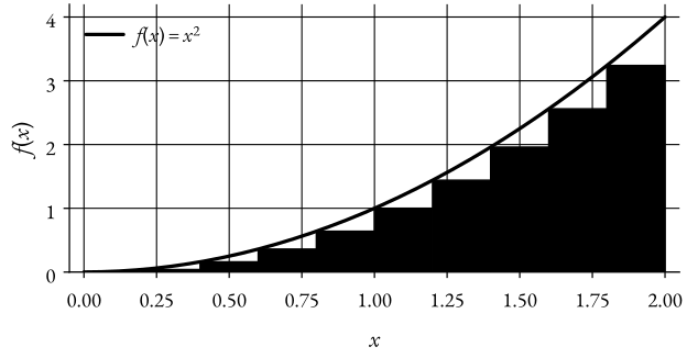
Figure 5: An example of a Riemann sum with n = 10 n = 10 n = 10 0.8 0.8 0.8 f ( x ) = x 2 f(x) = x^2 f ( x ) = x 2 How is convergence defined?
A deterministic sequence x n ∈ R x_n \in \mathbb{R} x n ∈ R a a a ∀ ϵ > 0 , ∃ N \forall \epsilon > 0, \exists N ∀ ϵ > 0 , ∃ N
∥ x n − a ∥ 2 < ϵ , ∀ n > N . \Vert x_n - a \Vert_2 < \epsilon, \quad \forall n > N. ∥ x n − a ∥ 2 < ϵ , ∀ n > N . That is, for sufficiently large n n n x n x_n x n a a a
How should one define convergence for a sequence of random variables?
A few (decently) intuitive ways are,
The sequence of random variables x n x_n x n x x x
with probability 1 (almost surely) if,
Pr [ lim n → ∞ x n ( ω ) = x ( ω ) ] = 1. \Pr[\lim_{n \to \infty} x_n(\omega) = x(\omega)] = 1. Pr [ n → ∞ lim x n ( ω ) = x ( ω )] = 1. lim n → ∞ E [ ( x n − x ) 2 ] = 0. \lim_{n \to \infty} \mathbb{E}[(x_n - x)^2] = 0. n → ∞ lim E [( x n − x ) 2 ] = 0.
in probability if for all ϵ > 0 \epsilon > 0 ϵ > 0
lim n → ∞ Pr [ ∥ x n ( ω ) − x ( ω ) ∥ ≥ ϵ ] = 0 , \lim_{n \to \infty} \Pr[\Vert x_n(\omega) - x(\omega) \Vert \geq \epsilon] = 0, n → ∞ lim Pr [ ∥ x n ( ω ) − x ( ω ) ∥ ≥ ϵ ] = 0 ,
in distribution if for all A ⊂ R n A \subset \mathbb{R}^n A ⊂ R n
lim n → ∞ Pr [ x n ∈ A ] = Pr [ x ∈ A ] . \lim_{n \to \infty} \Pr[x_n \in A] = \Pr[x \in A]. n → ∞ lim Pr [ x n ∈ A ] = Pr [ x ∈ A ] . The “weakest” of these is convergence in distribution, and the “strongest” is convergence almost surely.
Warning (Convergence in distribution) Suppose x , x 1 , x 2 , … x, x_1, x_2, \ldots x , x 1 , x 2 , … N ( 0 , 1 ) \mathcal{N}(0, 1) N ( 0 , 1 )
The random sequence only converges in distribution,
lim n → ∞ Pr [ x n ≤ a ] = Pr [ x ≤ a ] . \lim_{n \to \infty} \Pr[x_n \leq a] = \Pr[x \leq a]. n → ∞ lim Pr [ x n ≤ a ] = Pr [ x ≤ a ] . Warning (Convergence in almost surely, mean square, and in probability) Suppose x , y 1 , y 2 , … x, y_1, y_2, \ldots x , y 1 , y 2 , … N ( 0 , 1 ) \mathcal{N}(0, 1) N ( 0 , 1 )
The random sequence x n = x + y n n x_n = x + \frac{y_n}{n} x n = x + n y n x x x
Continuous and Differentiable Random Variables
Definition 3 (Definition: Continuous random functions (in mean square sense)) The random function is continuous in mean square at t t t
l.i.m h → 0 x ( t + h ) = x ( t ) , \underset{h \to 0}{\text{l.i.m}}\, x(t + h) = x(t), h → 0 l.i.m x ( t + h ) = x ( t ) , where l.i.m \text{l.i.m} l.i.m limits in mean square .
Definition 4 (Definition: Differentiable random functions (in mean square sense)) The mean square derivative is,
x ˙ ( t ) ≜ l.i.m h → 0 x ( t + h ) − x ( t ) h , \dot{x}(t) \triangleq \underset{h \to 0}{\text{l.i.m}} \frac{x(t + h) - x(t)}{h}, x ˙ ( t ) ≜ h → 0 l.i.m h x ( t + h ) − x ( t ) , if the limit exists.
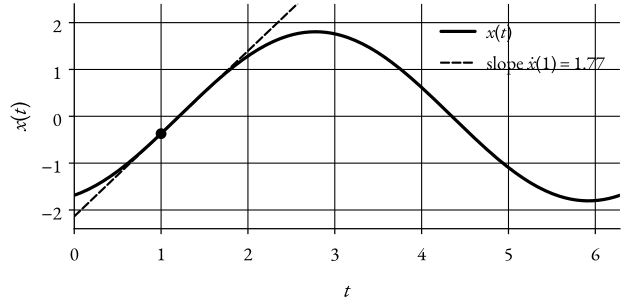
Figure 6: Visualization of a random differentiable function.Consider x ( t ) = a sin ( t + ϕ ) x(t) = a \sin(t + \phi) x ( t ) = a sin ( t + ϕ ) a ∼ unif [ 1 , 2 ] a \sim \text{unif}[1, 2] a ∼ unif [ 1 , 2 ] ϕ ∼ unif [ 0 , 2 π ] \phi \sim \text{unif}[0, 2\pi] ϕ ∼ unif [ 0 , 2 π ]
The random function is differentiable .
Note that the derivative is itself random.
See Figure 6 for a visualization of the random function and its derivative at x = 1 x = 1 x = 1
Definition 5 (Definition: Mean square Riemann integrals) Riemann integrals:
As before, let P ( t ) P(t) P ( t ) [ a , b ] [a, b] [ a , b ]
a = t 0 < t 1 < … < t n = b , a = t_0 < t_1 < \ldots < t_n = b, a = t 0 < t 1 < … < t n = b , and let its norm be ∣ P ∣ = max i ( t i + 1 − t i ) |P| = \underset{i}{\max}(t_{i+1} - t_i) ∣ P ∣ = i max ( t i + 1 − t i )
∫ a b x ( t ) d t ≜ l.i.m n → ∞ ∣ P ∣ → 0 ∑ i = 0 n − 1 ( t i + 1 − t i ) x ( t i ⋆ ) , \int_{a}^{b} x(t) \, dt \triangleq \underset{\substack{n \to \infty \newline |P| \to 0}}{\text{l.i.m}} \sum_{i=0}^{n-1} (t_{i+1} - t_i) x(t^{\star}_i), ∫ a b x ( t ) d t ≜ n → ∞ ∣ P ∣ → 0 l.i.m i = 0 ∑ n − 1 ( t i + 1 − t i ) x ( t i ⋆ ) , for any t i ⋆ ∈ [ t i , t i + 1 ] t^{\star}_i \in [t_i, t_{i+1}] t i ⋆ ∈ [ t i , t i + 1 ]
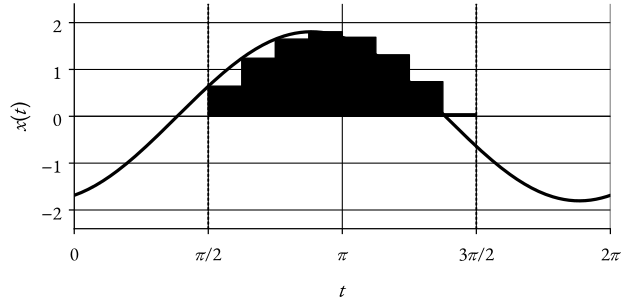
Figure 7: Visualization of a random integral.For x ( t ) = a sin ( t + ϕ ) x(t) = a \sin(t + \phi) x ( t ) = a sin ( t + ϕ )
∫ π 2 3 π 2 x ( t ) d t . \int_{\frac{\pi}{2}}^{\frac{3\pi}{2}} x(t) \, dt. ∫ 2 π 2 3 π x ( t ) d t . Note, the integral is a random variable.
Summary
Most SDEs take the form,
d x ( t ) = f ( x ( t ) , t ) d t ⏟ drift + L ( x ( t ) , t ) d β ( t ) ⏟ diffusion , \begin{equation}
dx(t) = \underbrace{f(x(t), t) \, dt}_{\text{drift}} + \underbrace{L(x(t), t) \, d\beta(t)}_{\text{diffusion}},
\end{equation} d x ( t ) = drift f ( x ( t ) , t ) d t + diffusion L ( x ( t ) , t ) d β ( t ) , where x ( t ) x(t) x ( t ) β ( t ) \beta(t) β ( t )
SDEs describe a class of stochastic processes useful in many areas (economics, physics, etc).
Where we specifically (will) focus on (deep) generative models.
We can use mean square convergence to define convergence, derivatives, and Riemann integrals for stochastic processes.
Equation (3) is shorthand for,
x ( t ) − x ( t 0 ) = ∫ t 0 t f ( x ( s ) , s ) d s + ∫ t 0 t L ( x ( s ) , s ) d β ( s ) . x(t) - x(t_0) = \int_{t_0}^t f(x(s), s) \, ds + \int_{t_0}^t L(x(s), s) \, d\beta(s). x ( t ) − x ( t 0 ) = ∫ t 0 t f ( x ( s ) , s ) d s + ∫ t 0 t L ( x ( s ) , s ) d β ( s ) . Note , we can use mean square Riemann integrals to define ∫ t 0 t f ( x ( s ) , s ) d s \int_{t_0}^{t} f(x(s), s) \, ds ∫ t 0 t f ( x ( s ) , s ) d s ∫ t 0 t L ( x ( s ) , s ) d β ( s ) \int_{t_0}^{t} L(x(s), s) \, d\beta(s) ∫ t 0 t L ( x ( s ) , s ) d β ( s )
We need Itô calc for that ;).