Part 2 - Brownian Motion and Itô Integrals

Introduction

Recall that we study SDEs of the form,

\begin{align*} dx(t) & = \underbrace{f(x(t), t) \ dt}_{\text{drift}} + \underbrace{L(x(t), t) \ d\beta(t)}_{\text{diffusion}}, \newline x(t) - x(t_0) & = \underbrace{\int_{t_0}^t f(x(s), s) \ ds}_{\text{mean square Riemann integral}} + \underbrace{\int_{t_0}^t L(x(s), s) \ d\beta(s)}_{\text{Itô integral}}. \end{align*}

where $x(t)$ is a stochastic process and $\beta(t)$ is a Brownian motion.

Today we’ll understand why the second integral will be solved with the Itô integral and not the (mean square) Riemann integral.

To understand this, let’s firstly study Brownian motion and its properties.

Brownian Motion

Recall the definition of Brownian motion,

Definition 1 (Definition: Brownian motion –

\beta(t)

)

Any increment $\Delta \beta(t) = \beta(t^{\prime}) - \beta(t) \sim \mathcal{N}(0, (t^{\prime} - t))$ .
Increments are independent unless intervals overlap.
$\beta(0) = 0$ .

We can see that the variance grows linearly with time, we can argue for this given independent and stationary intervals.

For an interval $[t_0, t_1, t_2]$ with $t_0 < t_1 < t_2$ , we have

\beta(t_2) - \beta(t_0) = \underbrace{\underbrace{\beta(t_2) - \beta(t_1)}_{\sim \mathcal{N}(0, (t_2 - t_1))} + \underbrace{\beta(t_1) - \beta(t_0)}_{\sim \mathcal{N}(0, (t_1 - t_0))}}_{\sim \mathcal{N}(0, (t_2 - t_0))},

which matches assumption (1) of Brownian motion.

In fact, the linear variance in (1) follows from stationary independent increments.

Is $\beta(t)$ a continuous?

Let’s investigate if $\beta(t)$ is continuous.

As we have seen previously, we can show that a random sequence is continuous (in mean square) if,

\begin{align*} \underset{h \to 0}{\text{l.i.m}} \ \beta(t + h) & = \beta(t), \newline \lim_{h \to 0} \mathbb{E}[\Vert \beta(t + h) - \beta(t) \Vert^2] & = 0. \end{align*}

By the definition of Brownian motion (and assumption (1)), we have

\begin{align*} \lim_{h \to 0} \mathbb{E}[\Vert \underbrace{\beta(t + h) - \beta(t)}_{\sim \mathcal{N}(0, |h|)} \Vert^2] & = \newline \lim_{h \to 0} |h| & = 0 \quad \square \end{align*}

Hence, $\beta(t)$ is continuous.

Is $\beta(t)$ differentiable?

Is there a random variable $\dot{\beta}(t)$ ,

\underset{h \to 0}{\text{l.i.m}} \ \frac{\beta(t + h) - \beta(t)}{h} = \dot{\beta}(t),

which is equivalent to,

\lim_{h \to 0} \mathbb{E}\left[\left\Vert \underbrace{\frac{\beta(t + h) - \beta(t)}{h}}_{\mathcal{N}(0, \frac{1}{|h|})} - \dot{\beta}(t) \right\Vert^2\right] = 0.

Since $\frac{\beta(t + h) - \beta(t)}{h} \sim \mathcal{N}(0, \frac{1}{|h|})$ , has a variance that grows with $|h|$ , we can see that the limit does not exist (goes to $\infty$ as $h \to 0$ ).

Instead, $\beta(t)$ is like a fractal as $h \to 0$ the variance grows to $\infty$ .

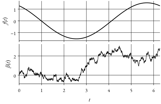A sinusoidal function VS. Brownian motion .

Properties of Brownian motion

Let’s summarize the properties of Brownian motion,

Note (Continuous but non-differentiable)

Brownian motion is (in mean square) continuous. It is also everywhere continuous with probability 1 (almost surely).
Brownian motion is mean square non-differentiable. It is also nowhere differentiable with probability 1 (almost surely).
A standard Brownian motion $(Q = 1)$ is often called a Wiener process [^1].
Brownian motion is a martingale [^2], $\mathbb{E}[x(t + \tau) | x(t)] = x(t)$ for $\tau > 0$ .
Brownian motion has independent and stationary increments and is the most famous Lévy process [^3].
It is Markovian, i.e., $p(x(t_i) | x(t_1), \ldots, x(t_{i-1})) = p(x(t_i) | x(t_{i-1}))$ if $t_j > t_{j_1}$ for all $j$ .
It is non-monotonic on all intervals, and it is a fractal.

Brownian motion and Riemann integral

A quick technical note, the Riemann-Stieltjes integral is defined as,

\int_{t_0}^{t_1} f(t) \ d\beta(t) = \lim_{n \to \infty} \sum_{i=0}^{n-1} f(t_i) (\beta(t_{i+1}) - \beta(t_i)),

you can see that the only difference is that the $(t_{i+1} - t_i)$ term is replaced with $(\beta(t_{i+1}) - \beta(t_i))$ .

So, why isn’t $\int_{t_0}^{t} L(x(s), s) \ d \beta(s)$ a Riemann-Stieltjes integral?

Let’s first recall the definition of the Riemann integral,

Definition 2 (Definition: Riemann integral)

If the limit exists, and is the same for any $t^{\star}_i \in [t_i, t_{i+1}]$ , the Riemann integral is defined as,

\int_{a}^{b} f(t) \ dt \triangleq \lim_{\substack{n \to \infty \newline |P| \to 0}} \sum_{i=0}^{n-1} (t_{i+1} - t_i) f(t^{\star}_i).

Suppose the limit exists for an arbitrary $t^{\star}_i \in [t_i, t_{i+1}]$ , do we get the same limit for $\forall t^{\star}_i \in [t_i, t_{i+1}]$ ?

Recall that $P(t)$ is a partition of $[a, b]: a = t_0 < t_1 < \ldots < t_n = b$ .

We assume that $t_{i + 1} = \frac{b - a}{n}$ for all $i \Rightarrow |P| = \underset{i}{\max}(t_{i + 1} - t_i) = \frac{b - a}{n}$ .

Left and Right Riemann sum

Let’s now investigate if the left and right Riemann sums have identical limits,

L(n) = \sum_{i=0}^{n-1} \underbrace{(t_{i + 1} - t_i)}_{= \frac{b - a}{n}} f(t_i) \quad \text{and} \quad R(n) = \sum_{i=0}^{n-1} \underbrace{(t_{i + 1} - t_i)}_{= \frac{b - a}{n}} f(t_{i + 1}).

We’ll investigate three different examples, starting with the (trivial) case.

Example 1: $f(t) = t$

Consider the case when $f(t) = t$ , we’ll denote $(t_{i + 1} - t_i) = \frac{b - a}{n} = \Delta t$ ,

\begin{align*} L(n) & = \sum_{i=0}^{n-1} \Delta t \cdot t_i, \newline R(n) & = \sum_{i=0}^{n-1} \Delta t \cdot t_{i + 1}, \newline R(n) - L(n) & = \sum_{i=0}^{n-1} \Delta t \cdot \underbrace{(t_{i + 1} - t_i)}_{= \Delta t} \newline & = \sum_{i=0}^{n-1} \Delta t^2 \newline & = n \cdot \Delta t^2 \newline & = \frac{(b - a)^2}{n} = \mathcal{O}\left(\frac{1}{n}\right). \end{align*}

Thus, as $n \to \infty$ , $R(n) - L(n) \to 0$ .

Example 2: $\int t \ d\beta(t)$

Consider the Riemann(-Stieltjes) sum,

\sum_{i=0}^{n-1} f(t^{\star}_i)(\beta(t_{i + 1}) - \beta(t_i)).

Since we now have a random sequence, we need to take the limit in mean square, or in other words, is $\underset{n \to \infty}{\text{l.i.m}} \ R(n) - L(n) = 0$ ?

Again, we let $\Delta \beta_i = \beta(t_{i + 1}) - \beta(t_i) \sim \mathcal{N}(0, \Delta t)$ , and we have,

\begin{align*} R(n) - L(n) & = \sum_{i=0}^{n-1} \underbrace{\Delta \beta_i}_{\sim \mathcal{N}(0, \Delta t)} \cdot \underbrace{(t_{i + 1} - t_i)}_{\Delta t} \newline & = \sum_{i=0}^{n-1} \underbrace{\Delta \beta_i \cdot \Delta t}_{\sim \mathcal{N}(0, \Delta t^3)} \newline & = \underbrace{n \cdot \Delta \beta_i \cdot \Delta t}_{\sim \mathcal{N}(0, n \Delta t^3)} = \mathcal{O}\left(\frac{1}{n^2}\right). \end{align*}

Thus, as $n \to \infty$ , $R(n) - L(n) \to 0$ and it is mean square Riemann(-Stieltjes) integrable.

Example 3: $\int \beta(t) \ d\beta(t)$

Finally, let’s consider the case when $f(t) = \beta(t)$ , we compare,

\begin{align*} L(n) & = \sum_{i=0}^{n-1} \beta(t_i) \Delta \beta_i, \newline R(n) & = \sum_{i=0}^{n-1} \beta(t_{i + 1}) \Delta \beta_i, \newline \end{align*}

where $\Delta \beta_i = \beta(t_{i + 1}) - \beta(t_i) \sim \mathcal{N}(0, \Delta t)$ .

Is $\underset{n \to \infty}{\text{l.i.m}} \ R(n) - L(n) = 0$ ?

We have,

\begin{align*} R(n) - L(n) & = \sum_{i=0}^{n-1} \Delta \beta_i \cdot \underbrace{(\beta(t_{i + 1}) - \beta(t_i))}_{\Delta \beta_i} \newline & = \sum_{i=0}^{n-1} \Delta \beta_i^2 \newline & \Rightarrow \mathbb{E}[R(n) - L(n)] = \sum_{i=0}^{n-1} \mathbb{E}[\Delta \beta_i^2] \newline & \Rightarrow \mathrm{Var}(\Delta \beta_i) = \mathbb{E}[\Delta \beta_i - \underbrace{\mathbb{E}[\Delta \beta_i]}_{= 0}]^2 \newline & \Rightarrow \mathbb{E}[\Delta \beta_i^2] = \mathrm{Var}(\Delta \beta_i) = \Delta t \newline & \Rightarrow \mathbb{E}[R(n) - L(n)] = n \cdot \Delta t = \boxed{b - a}. \end{align*}

Thus, as $n \to \infty$ , $R(n) - L(n) \to b - a$ and it is not mean square Riemann(-Stieltjes) integrable.

Itô integral

Riemann(-Stieltjes) sums cannot define $\int \beta(t) \ d\beta(t)$ since the limit depends on $t^{\star}_i$ .

Instead, we define the Itô integral as,

Definition 3 (Definition: Itô integrals)

We define the Itô integral (of the diffusion term) as,

\int_{t_0}^{t} L(x(s), s) \ d\beta(s) = \underset{\substack{n \to \infty \newline |P| \to 0}}{\text{l.i.m}} \sum_{i=0}^{n-1} L(x(t_i), t_i) (\beta(t_{i + 1}) - \beta(t_i)).

The difference compared to using Riemann(-Stieltjes) sums is that $t^{\star}_i = t_i$ .

We finally have our definition of our SDEs,

x(t) - x(t_0) = \underbrace{\int_{t_0}^t f(x(s), s) \ ds}_{\text{mean square Riemann integral}} + \underbrace{\int_{t_0}^t L(x(s), s) \ d\beta(s)}_{\text{Itô integral}}.

The Euler-Maruyama method

It is generally intractable to exactly simulate a process $x(t)$ described by an SDE,

\begin{equation} dx(t) = f(x(t), t) \ dt + L(x(t), t) \ d\beta(t). \end{equation}

The Euler-Maruyama method corresponds to the approximation,

dx(t) \approx f(x(t_i), t_i) \ dt + L(x(t_i), t_i) \ d\beta(t), \quad \forall t_i \in [t_i, t_{i + 1}].

Definition 4 (Definition: The Euler-Maruyama method)

To simulate $x(t)$ from Equation (1), draw $x(t_0) \sim p(x(t_0))$ and repeat for $i = 0, \ldots$ ,

Sample the Brownian motion, $\Delta \beta_i \sim \mathcal{N}(0, \Delta t)$ .
Predict the mean, $\hat{x}(t_{i + 1}) = x(t_i) + (t_{i + 1} - t_i) f(x(t_i), t_i)$ .
Sample the new state, $x(t_{i + 1}) = \hat{x}(t_{i + 1}) + L(x(t_i), t_i) \Delta \beta_i$ .

Second-Order Stochastic Integrals

We can also define the second-order stochastic integrals,

\int_{a}^{b} g(t) (d \beta(t))^2 \triangleq \underset{\substack{n \to \infty \newline |P| \to 0}}{\text{l.i.m}} \sum_{i=0}^{n-1} g(t_i) (\beta(t_{i + 1}) - \beta(t_i))^2.

If we set $g(t) = 1$ and standard $P$ , we get,

\begin{equation} \sum_{i=0}^{n-1} (\beta(t_{i + 1}) - \beta(t_i))^2, \end{equation}

Which we know has an expected value of $b - a$ .

Now, let $z_i = \beta(t_{i + 1}) - \beta(t_i) \sim \mathcal{N}(0, \Delta t)$ .

Equation (2) is $\Vert z \Vert^2$ , $\mathbb{E}[\Vert z \Vert^2] = b - a$ , and $\dim(z) = n$ .

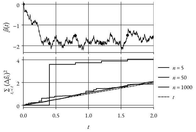Second-order stochastic integrals, as , the expected value of the sum converges to .

In a more abstract sense, as $n \to \infty$ , samples from $z$ concentrates close to the surface of a sphere.

This is known as concentration of measure ¹, a key result in many fields.

Note (Theorem on second-order stochastic integrals (scalar case))

Under suitable regularity conditions (e.g., g(t) is independent of future increments $\Delta \beta$ ),

\int_{a}^{b} g(t) (d \beta(t))^2 = \int_{a}^{b} g(t) dt.

In this context, we can simply replace (d $\beta(t)$ ) $^2$ by $dt$ and the Brownian motion does not introduce extra stochasticity.

Summary

Brownian motion can be defined by,

Definition 5 (Definition: Brownian motion –

\beta(t)

)

Any increment $\Delta \beta(t) = \beta(t^{\prime}) - \beta(t) \sim \mathcal{N}(0, (t^{\prime} - t))$ .
Increments are independent unless intervals overlap.
$\beta(0) = 0$ .

We have seen that $\beta(t)$ is continuous but non-differentiable.
Riemann(-Stieltjes) sums cannot be used to integrate, e.g., $\int \beta(t) \ d\beta(t)$ .
Instead, we normally use the Itô integral,

\int_{t_0}^{t} L(x(s), s) \ d\beta(s) \triangleq \underset{\substack{n \to \infty \newline |P| \to 0}}{\text{l.i.m}}\sum_{i=0}^{n-1} L(x(t_i), t_i) (\beta(t_{i + 1}) - \beta(t_i)).

The second-order stochastic integrals satisfy,

\int_{a}^{b} g(t) (d \beta(t))^2 = \int_{a}^{b} g(t) dt.

The Euler-Maruyama method is a simple sampling strategy, can be derived from,

dx(t) \approx f(x(t_i), t_i) \ dt + L(x(t_i), t_i) \ d\beta(t), \quad \forall t_i \in [t_i, t_{i + 1}].

Wikipedia: Concentration of measure ↩