Introduction
Recall that we study SDEs of the form,
d x ( t ) = f ( x ( t ) , t ) d t ⏟ drift + L ( x ( t ) , t ) d β ( t ) ⏟ diffusion , x ( t ) − x ( t 0 ) = ∫ t 0 t f ( x ( s ) , s ) d s ⏟ mean square Riemann Integral + ∫ t 0 t L ( x ( s ) , s ) d β ( s ) ⏟ It o ˆ Integral , \begin{align*}
dx(t) & = \underbrace{f(x(t), t) \, dt}_{\text{drift}} + \underbrace{L(x(t), t) \, d\beta(t)}_{\text{diffusion}}, \newline
x(t) - x(t_0) & = \underbrace{\int_{t_0}^{t} f(x(s), s) \, ds}_{\text{mean square Riemann Integral}} + \underbrace{\int_{t_0}^{t} L(x(s), s) \, d\beta(s)}_{\text{Itô Integral}},
\end{align*} d x ( t ) x ( t ) − x ( t 0 ) = drift f ( x ( t ) , t ) d t + diffusion L ( x ( t ) , t ) d β ( t ) , = mean square Riemann Integral ∫ t 0 t f ( x ( s ) , s ) d s + It o ˆ Integral ∫ t 0 t L ( x ( s ) , s ) d β ( s ) , where x ( t ) x(t) x ( t ) β ( t ) \beta(t) β ( t )
We define the Itô integral (of the diffusion term) as,
∫ t 0 t L ( x ( s ) , s ) d β ( s ) = l.i.m n → ∞ ∣ P ∣ → 0 ∑ i = 0 n − 1 L ( x ( t i ) , t i ) ( β ( t i + 1 ) − β ( t i ) ) . \int_{t_0}^{t} L(x(s), s) \, d\beta(s) = \underset{\substack{n \to \infty \newline |P| \to 0}}{\text{l.i.m}} \sum_{i=0}^{n-1} L(x(t_i), t_i) (\beta(t_{i + 1}) - \beta(t_i)). ∫ t 0 t L ( x ( s ) , s ) d β ( s ) = n → ∞ ∣ P ∣ → 0 l.i.m i = 0 ∑ n − 1 L ( x ( t i ) , t i ) ( β ( t i + 1 ) − β ( t i )) . Under suitable regularity conditions (e.g., f f f L L L 1 x ( t ) x(t) x ( t )
Note (Properties of SDEs)
The solution x ( t ) x(t) x ( t )
In short, x ( t ) x(t) x ( t ) not mean square differentiable .
The Classical Chain Rule
Suppose x ( t ) x(t) x ( t )
d x ( t ) d t = f ( x ( t ) ) . \frac{dx(t)}{dt} = f(x(t)). d t d x ( t ) = f ( x ( t )) . Definition 1 (Definition: The Chain Rule) If ϕ ( x ) \phi(x) ϕ ( x )
d ϕ ( x ( t ) ) d t = d ϕ ( x ( t ) ) d x ⏟ ϕ ′ ( x ( t ) ) d x ( t ) d t ⏟ x ′ ( t ) = ϕ ′ ( x ) f ( x ( t ) ) . \frac{d \phi(x(t))}{dt} = \underbrace{\frac{d \phi(x(t))}{dx}}_{\phi^{\prime}(x(t))} \underbrace{\frac{d x(t)}{dt}}_{x^{\prime}(t)} = \phi^{\prime}(x) f(x(t)). d t d ϕ ( x ( t )) = ϕ ′ ( x ( t )) d x d ϕ ( x ( t )) x ′ ( t ) d t d x ( t ) = ϕ ′ ( x ) f ( x ( t )) . Suppose x ( t ) x(t) x ( t )
d x ( t ) = f ( x ( t ) ) d t , x ( t ) − x ( t 0 ) = ∫ t 0 t f ( x ( s ) ) d s . \begin{align*}
dx(t) & = f(x(t)) \, dt, \newline
x(t) - x(t_0) & = \int_{t_0}^{t} f(x(s)) \, ds.
\end{align*} d x ( t ) x ( t ) − x ( t 0 ) = f ( x ( t )) d t , = ∫ t 0 t f ( x ( s )) d s . Definition 2 (Definition: The Chain Rule) If ϕ ( x ) \phi(x) ϕ ( x )
ϕ ( x ( t ) ) − ϕ ( x ( 0 ) ) = ∫ 0 t d ϕ ( x ( s ) ) d s d s = ∫ 0 t ϕ ′ ( x ( s ) ) d x ( s ) = ∫ 0 t ϕ ′ ( x ( s ) ) f ( x ( s ) ) d s , d ϕ ( x ( t ) ) = ϕ ′ ( x ( t ) ) d x ( t ) = ϕ ′ ( x ( t ) ) f ( x ( t ) ) d t . \begin{align*}
\phi(x(t)) - \phi(x(0)) & = \int_{0}^{t} \frac{d \phi(x(s))}{ds} \, ds = \int_{0}^{t} \phi^{\prime}(x(s)) \, dx(s) \newline
& = \int_{0}^{t} \phi^{\prime}(x(s)) f(x(s)) \, ds, \newline
d \phi(x(t)) & = \phi^{\prime}(x(t)) \, dx(t) = \phi^{\prime}(x(t)) f(x(t)) \, dt.
\end{align*} ϕ ( x ( t )) − ϕ ( x ( 0 )) d ϕ ( x ( t )) = ∫ 0 t d s d ϕ ( x ( s )) d s = ∫ 0 t ϕ ′ ( x ( s )) d x ( s ) = ∫ 0 t ϕ ′ ( x ( s )) f ( x ( s )) d s , = ϕ ′ ( x ( t )) d x ( t ) = ϕ ′ ( x ( t )) f ( x ( t )) d t . Consider a partition, a = t 0 < t 1 < … < t n = b a = t_0 < t_1 < \ldots < t_n = b a = t 0 < t 1 < … < t n = b t i + 1 − t i = Δ t = b − a n t_{i+1} - t_i = \Delta t = \frac{b - a}{n} t i + 1 − t i = Δ t = n b − a i = 0 , 1 , … , n − 1 i = 0, 1, \ldots, n - 1 i = 0 , 1 , … , n − 1
It follows that,
ϕ ( x ( b ) ) − ϕ ( x ( a ) ) = ∑ i = 0 n − 1 ϕ ( x ( t i + 1 ) ) − ϕ ( x ( t i ) ) . \phi(x(b)) - \phi(x(a)) = \sum_{i=0}^{n-1} \phi(x(t_{i + 1})) - \phi(x(t_i)). ϕ ( x ( b )) − ϕ ( x ( a )) = i = 0 ∑ n − 1 ϕ ( x ( t i + 1 )) − ϕ ( x ( t i )) . We have n n n Δ t = b − a n ⇒ O ( Δ t 2 ) \Delta t = \frac{b - a}{n} \Rightarrow \mathcal{O}(\Delta t^2) Δ t = n b − a ⇒ O ( Δ t 2 ) n → ∞ n \to \infty n → ∞
Using d x ( t ) = f ( x ( t ) ) d t dx(t) = f(x(t)) \, dt d x ( t ) = f ( x ( t )) d t
x ( t i + 1 ) = x ( t i ) + f ( x ( t i ) ) Δ t + O ( Δ t 2 ) , ϕ ( x ( t i + 1 ) ) = ϕ ( x ( t i ) ) + ϕ ′ ( x ( t i ) ) ( x ( t i + 1 ) − x ( t i ) ) + O ( Δ t 2 ) . \begin{align*}
x(t_{i + 1}) & = x(t_i) + f(x(t_i)) \Delta t + \mathcal{O}(\Delta t^2), \newline
\phi(x(t_{i + 1})) & = \phi(x(t_i)) + \phi^{\prime}(x(t_i))(x(t_{i + 1}) - x(t_i)) + \mathcal{O}(\Delta t^2).
\end{align*} x ( t i + 1 ) ϕ ( x ( t i + 1 )) = x ( t i ) + f ( x ( t i )) Δ t + O ( Δ t 2 ) , = ϕ ( x ( t i )) + ϕ ′ ( x ( t i )) ( x ( t i + 1 ) − x ( t i )) + O ( Δ t 2 ) . Thus, we conclude that,
ϕ ( x ( b ) ) − ϕ ( x ( a ) ) = ∑ i = 0 n − 1 ϕ ′ ( x ( t i ) ) f ( x ( t i ) ) Δ t = ∫ a b ϕ ′ ( x ( t ) ) f ( x ( t ) ) d t . \phi(x(b)) - \phi(x(a)) = \sum_{i=0}^{n-1} \phi^{\prime}(x(t_i)) f(x(t_i)) \Delta t = \int_{a}^{b} \phi^{\prime}(x(t)) f(x(t)) \, dt. ϕ ( x ( b )) − ϕ ( x ( a )) = i = 0 ∑ n − 1 ϕ ′ ( x ( t i )) f ( x ( t i )) Δ t = ∫ a b ϕ ′ ( x ( t )) f ( x ( t )) d t . Recall that the ODE d x ( t ) = f ( x ( t ) ) d t dx(t) = f(x(t)) \, dt d x ( t ) = f ( x ( t )) d t O ( Δ t 2 ) \mathcal{O}(\Delta t^2) O ( Δ t 2 ) n → ∞ n \to \infty n → ∞
d ϕ ( x ( t ) ) = ϕ ′ ( x ( t ) ) d x ( t ) + 1 2 ϕ ′ ′ ( x ( t ) ) ( d x ( t ) ) 2 + O ( ( d x ( t ) ) 3 ) = ϕ ′ ( x ( t ) ) d x ( t ) = ϕ ′ ( x ( t ) ) f ( x ( t ) ) d t . \begin{align*}
d\phi(x(t)) & = \phi^{\prime}(x(t)) \, dx(t) + \frac{1}{2} \phi^{\prime \prime}(x(t)) (dx(t))^2 + \mathcal{O}((dx(t))^3) \newline
& = \phi^{\prime}(x(t)) \, dx(t) \newline
& = \phi^{\prime}(x(t)) f(x(t)) \, dt.
\end{align*} d ϕ ( x ( t )) = ϕ ′ ( x ( t )) d x ( t ) + 2 1 ϕ ′′ ( x ( t )) ( d x ( t ) ) 2 + O (( d x ( t ) ) 3 ) = ϕ ′ ( x ( t )) d x ( t ) = ϕ ′ ( x ( t )) f ( x ( t )) d t . Solving ODEs
The chain rule is useful in various contexts, but we note that it yields a new ODE ,
d x ( t ) = f ( x ( t ) ) d t , d ϕ ( x ( t ) ) = ϕ ′ ( x ( t ) ) d x ( t ) = ϕ ′ ( x ( t ) ) f ( x ( t ) ) d t . \begin{align*}
dx(t) & = f(x(t)) \, dt, \newline
d\phi(x(t)) & = \phi^{\prime}(x(t)) \, dx(t) \newline
& = \phi^{\prime}(x(t)) f(x(t)) \, dt.
\end{align*} d x ( t ) d ϕ ( x ( t )) = f ( x ( t )) d t , = ϕ ′ ( x ( t )) d x ( t ) = ϕ ′ ( x ( t )) f ( x ( t )) d t . We can use this to solve ODEs.
Note (Example) Solving d x ( t ) = − c x ( t ) d t dx(t) = -cx(t) \, dt d x ( t ) = − c x ( t ) d t x ( 0 ) = 1 x(0) = 1 x ( 0 ) = 1
We introduce ϕ ( x ( t ) ) = log x ( t ) \phi(x(t)) = \log x(t) ϕ ( x ( t )) = log x ( t )
d ϕ ( x ( t ) ) = d x ( t ) x ( t ) = − c d t . d\phi(x(t)) = \frac{dx(t)}{x(t)} = -c \, dt. d ϕ ( x ( t )) = x ( t ) d x ( t ) = − c d t . This implies that ϕ ( x ( t ) ) = − c t \phi(x(t)) = -ct ϕ ( x ( t )) = − c t
x ( t ) = exp ( − c t ) . x(t) = \exp(-ct). x ( t ) = exp ( − c t ) . Itô Stochastic Calculus
Suppose x ( t ) x(t) x ( t )
d x ( t ) = f ( x ( t ) , t ) d t + L ( x ( t ) , t ) d β ( t ) . dx(t) = f(x(t), t) \, dt + L(x(t), t) \, d\beta(t). d x ( t ) = f ( x ( t ) , t ) d t + L ( x ( t ) , t ) d β ( t ) . The “chain rule” for ϕ ( x ( t ) ) \phi(x(t)) ϕ ( x ( t )) Itô formula .
To present a short derivation, we recall that,
∫ a b g ( t ) ( d β ( t ) ) 2 = ∫ a b g ( t ) d t . \int_{a}^{b} g(t) (d\beta(t))^2 = \int_{a}^{b} g(t) \, dt. ∫ a b g ( t ) ( d β ( t ) ) 2 = ∫ a b g ( t ) d t . It is also easy to verify that all other higher-order terms vanish, e.g.,
∫ a b g ( t ) d t d β ( t ) = 0. \int_{a}^{b} g(t) \, dt \, d\beta(t) = 0. ∫ a b g ( t ) d t d β ( t ) = 0. The Itô formula can thus be formally derived as,
d ϕ ( x ( t ) ) = ϕ ′ ( x ( t ) ) d x ( t ) + 1 2 ϕ ′ ′ ( x ( t ) ) ( d x ( t ) ) 2 + O ( ( d x ( t ) ) 3 ) = ϕ ′ ( x ( t ) ) ( f ( x ( t ) , t ) d t + L ( x ( t ) , t ) d β ( t ) ) + 1 2 ϕ ′ ′ ( x ( t ) ) ( L ( x ( t ) , t ) ) 2 d t . \begin{align*}
d \phi(x(t)) & = \phi^{\prime}(x(t)) \, dx(t) + \frac{1}{2} \phi^{\prime \prime}(x(t)) (dx(t))^2 + \mathcal{O}((dx(t))^3) \newline
& = \phi^{\prime}(x(t)) \left( f(x(t), t) \, dt + L(x(t), t) \, d\beta(t) \right) + \frac{1}{2} \phi^{\prime \prime}(x(t)) (L(x(t), t))^2 \, dt.
\end{align*} d ϕ ( x ( t )) = ϕ ′ ( x ( t )) d x ( t ) + 2 1 ϕ ′′ ( x ( t )) ( d x ( t ) ) 2 + O (( d x ( t ) ) 3 ) = ϕ ′ ( x ( t )) ( f ( x ( t ) , t ) d t + L ( x ( t ) , t ) d β ( t ) ) + 2 1 ϕ ′′ ( x ( t )) ( L ( x ( t ) , t ) ) 2 d t . The Itô formula can be generalized to vector-valued states and ϕ , f \phi, f ϕ , f L L L
Let’s present a scalar version where ϕ \phi ϕ ϕ ( x ( t ) , t ) \phi(x(t), t) ϕ ( x ( t ) , t )
Definition 3 (Definition: The Itô formula) Suppose x ( t ) x(t) x ( t )
d x ( t ) = f ( x ( t ) , t ) d t + L ( x ( t ) , t ) d β ( t ) . dx(t) = f(x(t), t) \, dt + L(x(t), t) \, d\beta(t). d x ( t ) = f ( x ( t ) , t ) d t + L ( x ( t ) , t ) d β ( t ) . The scalar function ϕ ( x ( t ) , t ) \phi(x(t), t) ϕ ( x ( t ) , t )
d ϕ ( x ( t ) , t ) = ∂ ϕ ∂ t d t + ∂ ϕ ∂ x d x ( t ) + 1 2 ∂ 2 ϕ ∂ x 2 L ( x ( t ) ) 2 d t . d \phi(x(t), t) = \frac{\partial \phi}{\partial t} dt + \frac{\partial \phi}{\partial x} dx(t) + \frac{1}{2} \frac{\partial^2 \phi}{\partial x^2} L(x(t))^2 dt. d ϕ ( x ( t ) , t ) = ∂ t ∂ ϕ d t + ∂ x ∂ ϕ d x ( t ) + 2 1 ∂ x 2 ∂ 2 ϕ L ( x ( t ) ) 2 d t . We can use this to solve SDEs.
Note (Example) Solving d x ( t ) = − c x ( t ) d t + x ( t ) d β ( t ) dx(t) = -cx(t) \, dt + x(t) \, d\beta(t) d x ( t ) = − c x ( t ) d t + x ( t ) d β ( t ) x ( 0 ) = 1 x(0) = 1 x ( 0 ) = 1
We introduce ϕ ( x ( t ) , t ) = log x ( t ) \phi(x(t), t) = \log x(t) ϕ ( x ( t ) , t ) = log x ( t )
d ϕ ( x ( t ) , t ) = d x ( t ) x ( t ) − ( d x ( t ) ) 2 2 ( x ( t ) ) 2 = − c d t + d β ( t ) − 1 2 d t . d \phi(x(t), t) = \frac{dx(t)}{x(t)} - \frac{(dx(t))^2}{2 (x(t))^2} = -c \, dt + d\beta(t) - \frac{1}{2} dt. d ϕ ( x ( t ) , t ) = x ( t ) d x ( t ) − 2 ( x ( t ) ) 2 ( d x ( t ) ) 2 = − c d t + d β ( t ) − 2 1 d t . This implies that ϕ ( x ( t ) , t ) = − ( c + 1 2 ) t + β ( t ) \phi(x(t), t) = -(c + \frac{1}{2}) t + \beta(t) ϕ ( x ( t ) , t ) = − ( c + 2 1 ) t + β ( t )
x ( t ) = exp ( − ( c + 1 2 ) t + β ( t ) ) . x(t) = \exp\left(-\left(c + \frac{1}{2}\right) t + \beta(t)\right). x ( t ) = exp ( − ( c + 2 1 ) t + β ( t ) ) . A Toy Example
Note (Example) Squared Brownian Motion
Suppose x ( 0 ) = 0 x(0) = 0 x ( 0 ) = 0 d x ( t ) = d β ( t ) dx(t) = d\beta(t) d x ( t ) = d β ( t ) x ( t ) = β ( t ) x(t) = \beta(t) x ( t ) = β ( t ) ϕ ( x ( t ) ) = x 2 ( t ) \phi(x(t)) = x^2(t) ϕ ( x ( t )) = x 2 ( t )
d ϕ ( x ( t ) ) = 2 x ( t ) d x ( t ) + ( d x ( t ) ) 2 = 2 β ( t ) d β ( t ) + d t . d \phi(x(t)) = 2 x(t) \, dx(t) + (dx(t))^2 = 2 \beta(t) \, d\beta(t) + dt. d ϕ ( x ( t )) = 2 x ( t ) d x ( t ) + ( d x ( t ) ) 2 = 2 β ( t ) d β ( t ) + d t . ⇒ ∫ 0 t d ϕ ( x ( s ) ) = β 2 ( t ) = ∫ 0 t 2 β ( s ) d β ( s ) + t . \Rightarrow \int_{0}^{t} d \phi(x(s)) = \beta^2(t) = \int_{0}^{t} 2 \beta(s) \, d\beta(s) + t. ⇒ ∫ 0 t d ϕ ( x ( s )) = β 2 ( t ) = ∫ 0 t 2 β ( s ) d β ( s ) + t . Note , for differentiable functions we get,
∫ 0 t f ( s ) d f ( s ) = ∫ 0 t f ( s ) f ′ ( s ) d s = 1 2 ∫ 0 t d f 2 ( s ) d s d s = f 2 ( t ) − f 2 ( 0 ) 2 , \int_{0}^{t} f(s) \, df(s) = \int_{0}^{t} f(s) f^{\prime}(s) \, ds = \frac{1}{2} \int_{0}^{t} \frac{d f^2(s)}{ds} \, ds = \frac{f^2(t) - f^2(0)}{2}, ∫ 0 t f ( s ) df ( s ) = ∫ 0 t f ( s ) f ′ ( s ) d s = 2 1 ∫ 0 t d s d f 2 ( s ) d s = 2 f 2 ( t ) − f 2 ( 0 ) , whereas the Itô formula yields an extra t t t
Starting from the SDE ( x ( t ) = β ( t ) ) (x(t) = \beta(t)) ( x ( t ) = β ( t ))
d x ( t ) = d β ( t ) , dx(t) = d\beta(t), d x ( t ) = d β ( t ) , we have derived an SDE for ϕ ( x ( t ) ) = β 2 ( t ) \phi(x(t)) = \beta^2(t) ϕ ( x ( t )) = β 2 ( t )
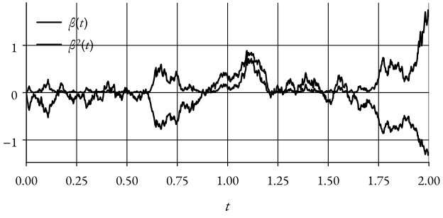
d ( β 2 ( t ) ) = 2 β ( t ) d β ( t ) + d t . d(\beta^2(t)) = 2 \beta(t) \, d\beta(t) + dt. d ( β 2 ( t )) = 2 β ( t ) d β ( t ) + d t . Figure 1: Brownian motion and its square.To verify the result, let us use the definition of the Itô integrals,
Note (Example: Squared Brownian Motion) The Itô formula implies that,
Using a partition, a = t 0 < t 1 < … < t n = b a = t_0 < t_1 < \ldots < t_n = b a = t 0 < t 1 < … < t n = b
∑ i = 0 n − 1 ( β 2 ( t i + 1 ) − β 2 ( t i ) ) ⏟ a 2 − b 2 = ∑ i = 0 n − 1 ( β ( t i + 1 ) + β ( t i ) ) ( β ( t i + 1 ) − β ( t i ) ) = ∑ i = 0 n − 1 2 β ( t i ) ( β ( t i + 1 ) − β ( t i ) ) + ( β ( t i + 1 ) − β ( t i ) ) 2 . \begin{align*}
\sum_{i=0}^{n-1} \underbrace{(\beta^2(t_{i + 1}) - \beta^2(t_i))}_{a^2 - b^2} & = \sum_{i=0}^{n-1} (\beta(t_{i + 1}) + \beta(t_i)) (\beta(t_{i + 1}) - \beta(t_i)) \newline
& = \sum_{i=0}^{n-1} 2 \beta(t_i) (\beta(t_{i + 1}) - \beta(t_i)) + (\beta(t_{i + 1}) - \beta(t_i))^2.
\end{align*} i = 0 ∑ n − 1 a 2 − b 2 ( β 2 ( t i + 1 ) − β 2 ( t i )) = i = 0 ∑ n − 1 ( β ( t i + 1 ) + β ( t i )) ( β ( t i + 1 ) − β ( t i )) = i = 0 ∑ n − 1 2 β ( t i ) ( β ( t i + 1 ) − β ( t i )) + ( β ( t i + 1 ) − β ( t i ) ) 2 . This converges (in mean square) to the right-hand side of Equation (1) as n → ∞ n \to \infty n → ∞
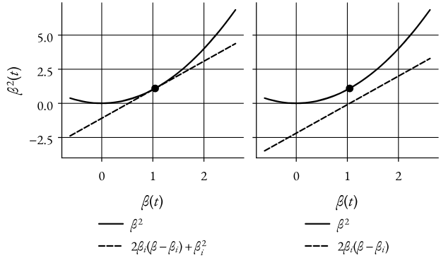
We can also visualize the nonlinear function ϕ ( x ( t ) ) \phi(x(t)) ϕ ( x ( t )) x ( t ) x(t) x ( t )
Note (Example: Squared Brownian Motion (cont’d)) We visualize β 2 ( t ) \beta^2(t) β 2 ( t ) β ( t ) \beta(t) β ( t )
Sum of the previous two integrals is the second-order Taylor expansion with respect to β ( t i + 1 ) \beta(t_{i + 1}) β ( t i + 1 )
The quadratic term converges in mean square to b − a = t b - a = t b − a = t n → ∞ n \to \infty n → ∞
Figure 2: Squared Brownian motion as a function of Brownian motion.
Notice how the quadratic term ensures that the Taylor expansion converges to the point heightwise.Vector Version
Consider a multi-dimensional SDE,
d x ( t ) = f ( x ( t ) , t ) d t + L ( x ( t ) , t ) d β ( t ) , d\mathbf{x}(t) = \mathbf{f}(\mathbf{x}(t), t) \, dt + \mathbf{L}(\mathbf{x}(t), t) \, d\beta(t), d x ( t ) = f ( x ( t ) , t ) d t + L ( x ( t ) , t ) d β ( t ) , where x \mathbf{x} x f \mathbf{f} f n × 1 n \times 1 n × 1 L \mathbf{L} L n × m n \times m n × m β ( t ) \beta(t) β ( t ) m × 1 m \times 1 m × 1
It follows that,
d ϕ ( x ( t ) , t ) = ∂ ϕ ( x ( t ) , t ) ∂ t d t + ∑ i ∂ ϕ ( x ( t ) , t ) ∂ x i ( t ) d x i ( t ) + 1 2 ∑ i , j ∂ 2 ϕ ( x ( t ) , t ) ∂ x i ( t ) ∂ x j ( t ) d x i ( t ) d x j ( t ) . \begin{align*}
d \phi(\mathbf{x}(t), t) = {} & \frac{\partial \phi(\mathbf{x}(t), t)}{\partial t} dt + \sum_i \frac{\partial \phi(\mathbf{x}(t), t)}{\partial x_i(t)} dx_i(t) \newline
& + \frac{1}{2} \sum_{i,j} \frac{\partial^2 \phi(\mathbf{x}(t), t)}{\partial x_i(t) \partial x_j(t)} dx_i(t) \, d x_j(t).
\end{align*} d ϕ ( x ( t ) , t ) = ∂ t ∂ ϕ ( x ( t ) , t ) d t + i ∑ ∂ x i ( t ) ∂ ϕ ( x ( t ) , t ) d x i ( t ) + 2 1 i , j ∑ ∂ x i ( t ) ∂ x j ( t ) ∂ 2 ϕ ( x ( t ) , t ) d x i ( t ) d x j ( t ) . All higher-order terms vanish except ( d β ( t ) ) 2 = d t (d\beta(t))^2 = dt ( d β ( t ) ) 2 = d t
We can express the relation on a more compact form,
d ϕ ( x ( t ) , t ) = ∂ ϕ ( x ( t ) , t ) ∂ t d t + ∑ i ∂ ϕ ( x ( t ) , t ) ∂ x i ( t ) d x i ( t ) + 1 2 ∑ i , j ∂ 2 ϕ ( x ( t ) , t ) ∂ x i ( t ) ∂ x j ( t ) d x i ( t ) d x j ( t ) = ∂ ϕ ∂ t d t + ( ∇ x ϕ ) T d x ( t ) + 1 2 d x ( t ) T ∇ x ∇ x T ϕ d x ( t ) . \begin{align*}
d \phi(\mathbf{x}(t), t) & = \frac{\partial \phi(\mathbf{x}(t), t)}{\partial t} dt + \sum_i \frac{\partial \phi(\mathbf{x}(t), t)}{\partial x_i(t)} dx_i(t) \newline
& \quad + \frac{1}{2} \sum_{i,j} \frac{\partial^2 \phi(\mathbf{x}(t), t)}{\partial x_i(t) \partial x_j(t)} dx_i(t) \, d x_j(t) \newline
& = \frac{\partial \phi}{\partial t} dt + (\nabla_{\mathbf{x}} \phi)^T d\mathbf{x}(t) + \frac{1}{2} d\mathbf{x}(t)^T \nabla_{\mathbf{x}} \nabla_{\mathbf{x}}^T \phi \, d\mathbf{x}(t).
\end{align*} d ϕ ( x ( t ) , t ) = ∂ t ∂ ϕ ( x ( t ) , t ) d t + i ∑ ∂ x i ( t ) ∂ ϕ ( x ( t ) , t ) d x i ( t ) + 2 1 i , j ∑ ∂ x i ( t ) ∂ x j ( t ) ∂ 2 ϕ ( x ( t ) , t ) d x i ( t ) d x j ( t ) = ∂ t ∂ ϕ d t + ( ∇ x ϕ ) T d x ( t ) + 2 1 d x ( t ) T ∇ x ∇ x T ϕ d x ( t ) . Using the expression for the SDE,
d ϕ ( x ( t ) , t ) = ∂ ϕ ∂ t d t + ( ∇ x ϕ ) T d x ( t ) + 1 2 d β T L T ∇ x ∇ x T ϕ L d β = ∂ ϕ ∂ t d t + ( ∇ x ϕ ) T d x ( t ) + 1 2 tr { L T ∇ x ∇ x T ϕ L } d t . \begin{align*}
d \phi(\mathbf{x}(t), t) & = \frac{\partial \phi}{\partial t} dt + (\nabla_{\mathbf{x}} \phi)^T d \mathbf{x}(t) + \frac{1}{2} d \beta^T \mathbf{L}^T \nabla_{\mathbf{x}} \nabla_{\mathbf{x}}^T \phi \mathbf{L} \, d\beta \newline
& = \frac{\partial \phi}{\partial t} dt + (\nabla_{\mathbf{x}} \phi)^T d \mathbf{x}(t) + \frac{1}{2} \operatorname{tr} \{\mathbf{L}^T \nabla_{\mathbf{x}} \nabla_{\mathbf{x}}^T \phi \mathbf{L} \} dt.
\end{align*} d ϕ ( x ( t ) , t ) = ∂ t ∂ ϕ d t + ( ∇ x ϕ ) T d x ( t ) + 2 1 d β T L T ∇ x ∇ x T ϕ L d β = ∂ t ∂ ϕ d t + ( ∇ x ϕ ) T d x ( t ) + 2 1 tr { L T ∇ x ∇ x T ϕ L } d t . Definition 4 (Definition: The Itô formula for vector states) Consider a multi-dimensional SDE,
d x ( t ) = f ( x ( t ) , t ) d t + L ( x ( t ) , t ) d β ( t ) , d\mathbf{x}(t) = \mathbf{f}(\mathbf{x}(t), t) \, dt + \mathbf{L}(\mathbf{x}(t), t) \, d\beta(t), d x ( t ) = f ( x ( t ) , t ) d t + L ( x ( t ) , t ) d β ( t ) , where x \mathbf{x} x f \mathbf{f} f n × 1 n \times 1 n × 1 L \mathbf{L} L n × m n \times m n × m β ( t ) \beta(t) β ( t ) m × 1 m \times 1 m × 1 ϕ ( x ( t ) , t ) \phi(\mathbf{x}(t), t) ϕ ( x ( t ) , t )
d ϕ ( x ( t ) , t ) = ∂ ϕ ∂ t d t + ( ∇ x ϕ ) T d x ( t ) + 1 2 tr { L T ∇ x ∇ x T ϕ L } d t . d \phi(\mathbf{x}(t), t) = \frac{\partial \phi}{\partial t} dt + (\nabla_{\mathbf{x}} \phi)^T d \mathbf{x}(t) + \frac{1}{2} \operatorname{tr} \{\mathbf{L}^T \nabla_{\mathbf{x}} \nabla_{\mathbf{x}}^T \phi \mathbf{L} \} dt. d ϕ ( x ( t ) , t ) = ∂ t ∂ ϕ d t + ( ∇ x ϕ ) T d x ( t ) + 2 1 tr { L T ∇ x ∇ x T ϕ L } d t . Stratonovich SDEs
Most SDEs are described using Itô integrals,
∫ a b L ( x ( t ) ) d β ( t ) ≜ l.i.m n → ∞ ∑ i = 0 n − 1 L ( x ( t i ) ) ( β ( t i + 1 ) − β ( t i ) ) , \int_{a}^{b} L(x(t)) \, d\beta(t) \triangleq \underset{n \to \infty}{\text{l.i.m}} \sum_{i=0}^{n-1} L(x(t_i)) (\beta(t_{i + 1}) - \beta(t_i)), ∫ a b L ( x ( t )) d β ( t ) ≜ n → ∞ l.i.m i = 0 ∑ n − 1 L ( x ( t i )) ( β ( t i + 1 ) − β ( t i )) , but it is not the only option.
Definition 5 (Definition: The Stratonovich Integral) The stochastic integral of Stratonovich is defined as,
∫ a b L ( x ( t ) ) ∘ d β ( t ) = l.i.m n → ∞ ∑ i = 0 n − 1 L ( x ( t i + 1 ) ) + L ( x ( t i ) ) 2 ( β ( t i + 1 ) − β ( t i ) ) . \int_{a}^{b} L(x(t)) \circ d\beta(t) = \underset{n \to \infty}{\text{l.i.m}} \sum_{i=0}^{n-1} \frac{L(x(t_{i + 1})) + L(x(t_i))}{2} (\beta(t_{i + 1}) - \beta(t_i)). ∫ a b L ( x ( t )) ∘ d β ( t ) = n → ∞ l.i.m i = 0 ∑ n − 1 2 L ( x ( t i + 1 )) + L ( x ( t i )) ( β ( t i + 1 ) − β ( t i )) . One advantage of Stratonovich is that the chain rule holds!
Stratonovich VS. Itô
Note (Converting SDEs) The Stratonovich SDE,
d x ( t ) = f ( x ( t ) ) d t + L ( x ( t ) ) ∘ d β ( t ) , dx(t) = f(x(t)) \, dt + L(x(t)) \circ d\beta(t), d x ( t ) = f ( x ( t )) d t + L ( x ( t )) ∘ d β ( t ) , is equivalent to the Itô SDE,
d x ( t ) = ( f ( x ( t ) ) + 1 2 L ′ ( x ( t ) ) L ( x ( t ) ) ) d t + L ( x ( t ) ) d β ( t ) . dx(t) = \left( f(x(t)) + \frac{1}{2} L^{\prime}(x(t)) L(x(t)) \right) dt + L(x(t)) \, d\beta(t). d x ( t ) = ( f ( x ( t )) + 2 1 L ′ ( x ( t )) L ( x ( t )) ) d t + L ( x ( t )) d β ( t ) . Hence, we can use results from Itô SDEs (e.g., Euler-Maruyama or the Itô formula) also on Stratonovich SDEs.
We will always assume Itô SDEs, but for completeness, one can write, e.g., “in the Itô sense” or “in the Stratonovich sense”.
Sketch of Proof
Consider the Stratonovich SDE,
d x ( t ) = f ( x ( t ) ) d t + L ( x ( t ) ) ∘ d β ( t ) . dx(t) = f(x(t)) \, dt + L(x(t)) \circ d\beta(t). d x ( t ) = f ( x ( t )) d t + L ( x ( t )) ∘ d β ( t ) . The conversion to an Itô SDE follows from (Δ β i ≜ β ( t i + 1 ) − β ( t i ) \Delta \beta_i \triangleq \beta(t_{i + 1}) - \beta(t_i) Δ β i ≜ β ( t i + 1 ) − β ( t i )
∫ L ( x ( t ) ) ∘ d β ( t ) = l.i.m n → ∞ ∑ i = 0 n − 1 L ( x ( t i + 1 ) ) + L ( x ( t i ) ) 2 Δ β i {Taylor Expansion} = l.i.m n → ∞ ∑ i = 0 n − 1 ( L ( x ( t i ) ) + 1 2 L ′ ( x ( t i ) ) ( x ( t i + 1 ) − x ( t i ) ) ) Δ β i = l.i.m n → ∞ ∑ i = 0 n − 1 L ( x ( t i ) ) Δ β i + 1 2 L ′ ( x ( t i ) ) L ( x ( t i ) ) Δ β i 2 . \begin{align*}
\int L(x(t)) \circ d\beta(t) & = \underset{n \to \infty}{\text{l.i.m}} \sum_{i=0}^{n-1} \frac{L(x(t_{i + 1})) + L(x(t_i))}{2} \Delta \beta_i \newline
\text{\{Taylor Expansion\}} & = \underset{n \to \infty}{\text{l.i.m}} \sum_{i=0}^{n-1} \left( L(x(t_i)) + \frac{1}{2} L^{\prime}(x(t_i))(x(t_{i + 1}) - x(t_i)) \right) \Delta \beta_i \newline
& = \underset{n \to \infty}{\text{l.i.m}} \sum_{i=0}^{n-1} L(x(t_i)) \Delta \beta_i + \frac{1}{2} L^{\prime}(x(t_i)) L(x(t_i)) \Delta \beta_i^2.
\end{align*} ∫ L ( x ( t )) ∘ d β ( t ) {Taylor Expansion} = n → ∞ l.i.m i = 0 ∑ n − 1 2 L ( x ( t i + 1 )) + L ( x ( t i )) Δ β i = n → ∞ l.i.m i = 0 ∑ n − 1 ( L ( x ( t i )) + 2 1 L ′ ( x ( t i )) ( x ( t i + 1 ) − x ( t i )) ) Δ β i = n → ∞ l.i.m i = 0 ∑ n − 1 L ( x ( t i )) Δ β i + 2 1 L ′ ( x ( t i )) L ( x ( t i )) Δ β i 2 . Summary
Definition 6 (Definition: The Itô formula) Suppose x ( t ) x(t) x ( t )
d x ( t ) = f ( x ( t ) , t ) d t + L ( x ( t ) , t ) d β ( t ) . dx(t) = f(x(t), t) \, dt + L(x(t), t) \, d\beta(t). d x ( t ) = f ( x ( t ) , t ) d t + L ( x ( t ) , t ) d β ( t ) . The scalar function ϕ ( x ( t ) , t ) \phi(x(t), t) ϕ ( x ( t ) , t )
d ϕ ( x ( t ) , t ) = ∂ ϕ ∂ t d t + ∂ ϕ ∂ x d x ( t ) + 1 2 ∂ 2 ϕ ∂ x 2 L ( x ( t ) ) 2 d t . d \phi(x(t), t) = \frac{\partial \phi}{\partial t} dt + \frac{\partial \phi}{\partial x} dx(t) + \frac{1}{2} \frac{\partial^2 \phi}{\partial x^2} L(x(t))^2 dt. d ϕ ( x ( t ) , t ) = ∂ t ∂ ϕ d t + ∂ x ∂ ϕ d x ( t ) + 2 1 ∂ x 2 ∂ 2 ϕ L ( x ( t ) ) 2 d t . The Itô formula is essential for understanding and working with SDEs.