SDEs and Probability Distributions
As always, we study SDEs of the form,
d x ( t ) = f ( x ( t ) , t ) d t ⏟ drift + L ( x ( t ) , t ) d β ( t ) ⏟ diffusion , dx(t) = \underbrace{f(x(t), t) \, dt}_{\text{drift}} + \underbrace{L(x(t), t) \, d\beta(t)}_{\text{diffusion}}, d x ( t ) = drift f ( x ( t ) , t ) d t + diffusion L ( x ( t ) , t ) d β ( t ) , where x ( t ) x(t) x ( t ) β ( t ) \beta(t) β ( t )
At each time t t t x ( t ) x(t) x ( t ) p ( x ( t ) , t ) p(x(t), t) p ( x ( t ) , t ) x ( t 0 ) ∼ p ( x ( t 0 ) , t 0 ) = p init ( x ( t 0 ) ) x(t_0) \sim p(x(t_0), t_0) = p_{\text{init}}(x(t_0)) x ( t 0 ) ∼ p ( x ( t 0 ) , t 0 ) = p init ( x ( t 0 ))
How does p ( x ( t ) , t ) p(x(t), t) p ( x ( t ) , t ) t ≥ t 0 t \geq t_0 t ≥ t 0
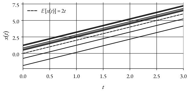
SDE with only drift
Figure 1: SDE with only drift (an ODE)Suppose f ( x ( t ) , t ) = 2 , L ( x ( t ) , t ) = 0 ⇒ d x d t = 2. f(x(t), t) = 2, L(x(t), t) = 0 \Rightarrow \frac{dx}{dt} = 2. f ( x ( t ) , t ) = 2 , L ( x ( t ) , t ) = 0 ⇒ d t d x = 2.
We also assume that x ( t 0 = 0 ) ∼ N ( 0 , 1 ) x(t_0 = 0) \sim \mathcal{N}(0, 1) x ( t 0 = 0 ) ∼ N ( 0 , 1 )
Intuitively, for this SDE (or ODE in this case), the probability distribution of x ( t ) x(t) x ( t )
x ( t ) ∼ N ( 2 t , 1 ) . x(t) \sim \mathcal{N}(2t, 1). x ( t ) ∼ N ( 2 t , 1 ) . But, more formally we know that,
x ( t ) = x ( 0 ) ⏟ N ( 0 , 1 ) + 2 t ⇒ x ( t ) ∼ N ( 2 t , 1 ) . \begin{align*}
x(t) & = \underbrace{x(0)}_{\mathcal{N}(0, 1)} + 2t \newline
& \Rightarrow x(t) \sim \mathcal{N}(2t, 1).
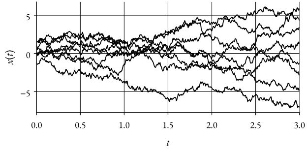
\end{align*} x ( t ) = N ( 0 , 1 ) x ( 0 ) + 2 t ⇒ x ( t ) ∼ N ( 2 t , 1 ) . SDE with only diffusion
Figure 2: SDE with only diffusionSuppose f ( x ( t ) , t ) = 0 , L ( x ( t ) , t ) = 2 ⇒ d x = 2 d β ( t ) f(x(t), t) = 0, L(x(t), t) = 2 \Rightarrow dx = 2 \, d\beta(t) f ( x ( t ) , t ) = 0 , L ( x ( t ) , t ) = 2 ⇒ d x = 2 d β ( t )
We also assume that x ( t 0 = 0 ) ∼ N ( 0 , 1 ) x(t_0 = 0) \sim \mathcal{N}(0, 1) x ( t 0 = 0 ) ∼ N ( 0 , 1 )
Thus,
x ( t ) = x ( 0 ) ⏟ N ( 0 , 1 ) + 2 β ( t ) ⏟ N ( 0 , 4 t ) ⇒ x ( t ) ∼ N ( 0 , 1 + 4 t ) . \begin{align*}
x(t) & = \underbrace{x(0)}_{\mathcal{N}(0, 1)} + \underbrace{2 \beta(t)}_{\mathcal{N}(0, 4t)} \newline
& \Rightarrow x(t) \sim \mathcal{N}(0, 1 + 4t).
\end{align*} x ( t ) = N ( 0 , 1 ) x ( 0 ) + N ( 0 , 4 t ) 2 β ( t ) ⇒ x ( t ) ∼ N ( 0 , 1 + 4 t ) . Connection to (Deep) Diffusion Models
So, we have seen that (simple) SDEs and their probability distributions evolve over time .
This is the key idea behind diffusion models.
Suppose x ( 0 ) ∼ p ( x ( 0 ) , 0 ) = p init ( x ( 0 ) ) x(0) \sim p(x(0), 0) = p_{\text{init}}(x(0)) x ( 0 ) ∼ p ( x ( 0 ) , 0 ) = p init ( x ( 0 )) p init p_{\text{init}} p init x ( 1 ) ∼ p ( x ( 1 ) , 1 ) = p data ( x ( 1 ) ) x(1) \sim p(x(1), 1) = p_{\text{data}}(x(1)) x ( 1 ) ∼ p ( x ( 1 ) , 1 ) = p data ( x ( 1 )) p data p_{\text{data}} p data
Can we and how do we construct such an SDE? If it is possible, then we can sample from p init p_{\text{init}} p init p data p_{\text{data}} p data
Fokker-Planck-Kolmogorov Equation
The Fokker-Planck-Kolmogorov equation describes the evolution of the probability distribution of a stochastic process over time,
Definition 1 (Definition: Fokker-Planck-Kolmogorov Equation in R d \mathbb{R}^d R d The probability density p ( x , t ) p(\mathbf{x}, t) p ( x , t )
d x ( t ) = f ( x ( t ) , t ) d t + L ( x ( t ) , t ) d β ( t ) , d\mathbf{x}(t) = \mathbf{f}(\mathbf{x}(t), t) \, dt + \mathbf{L}(\mathbf{x}(t), t) \, d\beta(t), d x ( t ) = f ( x ( t ) , t ) d t + L ( x ( t ) , t ) d β ( t ) , solves the partial differential equation,
∂ p ( x , t ) ∂ t = − ∑ i ∂ ∂ x i [ f i ( x , t ) p ( x , t ) ] + 1 2 ∑ i , j ∂ 2 ∂ x i ∂ x j [ [ L ( x , t ) L T ( x , t ) ] i j p ( x , t ) ] . \frac{\partial p(\mathbf{x}, t)}{\partial t} = - \sum_i \frac{\partial}{\partial x_i} [f_i(\mathbf{x}, t) p(\mathbf{x}, t)] + \frac{1}{2} \sum_{i,j} \frac{\partial^2}{\partial x_i \partial x_j} \left[ [\mathbf{L}(\mathbf{x}, t) \mathbf{L}^T(\mathbf{x}, t)]_{ij} p(\mathbf{x}, t) \right]. ∂ t ∂ p ( x , t ) = − i ∑ ∂ x i ∂ [ f i ( x , t ) p ( x , t )] + 2 1 i , j ∑ ∂ x i ∂ x j ∂ 2 [ [ L ( x , t ) L T ( x , t ) ] ij p ( x , t ) ] . In physics literature, this is often called the Fokker-Planck equation , while in stochastics, it is called the forward Kolmogorov equation .
Definition 2 (Definition: Fokker-Planck-Kolmogorov Equation in R \mathbb{R} R The probability density p ( x , t ) p(x, t) p ( x , t )
d x ( t ) = f ( x ( t ) , t ) d t + L ( x ( t ) , t ) d β ( t ) , dx(t) = f(x(t), t) \, dt + L(x(t), t) \, d\beta(t), d x ( t ) = f ( x ( t ) , t ) d t + L ( x ( t ) , t ) d β ( t ) , solves the partial differential equation,
∂ p ( x , t ) ∂ t = − ∂ ∂ x [ f ( x , t ) p ( x , t ) ] + 1 2 ∂ 2 ∂ x 2 [ L ( x , t ) 2 p ( x , t ) ] . \frac{\partial p(x, t)}{\partial t} = - \frac{\partial}{\partial x} [f(x, t) p(x, t)] + \frac{1}{2} \frac{\partial^2}{\partial x^2} \left[ L(x, t)^2 p(x, t) \right]. ∂ t ∂ p ( x , t ) = − ∂ x ∂ [ f ( x , t ) p ( x , t )] + 2 1 ∂ x 2 ∂ 2 [ L ( x , t ) 2 p ( x , t ) ] . Example: Diffusion
Let’s consider the SDE,
d x ( t ) = d β ( t ) , dx(t) = d \beta(t), d x ( t ) = d β ( t ) , Using the Fokker-Planck-Kolmogorov equation, we can derive the corresponding PDE,
∂ p ( x , t ) ∂ t = 1 2 ∂ 2 ∂ x 2 p ( x , t ) . \frac{\partial p(x, t)}{\partial t} = \frac{1}{2} \frac{\partial^2}{\partial x^2} p(x, t). ∂ t ∂ p ( x , t ) = 2 1 ∂ x 2 ∂ 2 p ( x , t ) . This is known as the diffusion or heat equation.
Fokker-Planck-Kolmogorov PDE Proof
We will prove the Fokker-Planck-Kolmogorov PDE, but let’s first understand some useful results that we’ll use.
Note (Integration by parts) ∫ a b u ′ ( x ) v ( x ) d x = [ u ( x ) v ( x ) ] a b − ∫ a b u ( x ) v ′ ( x ) d x . \int_{a}^{b} u^{\prime}(x) v(x) \, dx = [u(x) v(x)]_{a}^{b} - \int_{a}^{b} u(x) v^{\prime}(x) \, dx. ∫ a b u ′ ( x ) v ( x ) d x = [ u ( x ) v ( x ) ] a b − ∫ a b u ( x ) v ′ ( x ) d x . In higher dimensions it is known as the divergence theorem or Gauss’s theorem .
(This is nothing new, just a friendly reminder.)
Note (The Itô Formula) Suppose x ( t ) x(t) x ( t )
d x ( t ) = f ( x ( t ) , t ) d t + L ( x ( t ) , t ) d β ( t ) . dx(t) = f(x(t), t) \, dt + L(x(t), t) \, d\beta(t). d x ( t ) = f ( x ( t ) , t ) d t + L ( x ( t ) , t ) d β ( t ) . The scalar function ϕ ( x ) \phi(x) ϕ ( x ) t t t
d ϕ ( x ) = ∂ ϕ ∂ x d x + 1 2 ∂ 2 ϕ ∂ x 2 L ( x , t ) 2 d t . d\phi(x) = \frac{\partial \phi}{\partial x} dx + \frac{1}{2} \frac{\partial^2 \phi}{\partial x^2} L(x, t)^2 \, dt. d ϕ ( x ) = ∂ x ∂ ϕ d x + 2 1 ∂ x 2 ∂ 2 ϕ L ( x , t ) 2 d t . Taking the expectation and dividing by d t dt d t
d E [ ϕ ] d t = E [ ∂ ϕ ∂ x f ( x , t ) ] + 1 2 E [ ∂ 2 ϕ ∂ x 2 L ( x , t ) 2 ] . \frac{d \mathbb{E}[\phi]}{dt} = \mathbb{E}\left[ \frac{\partial \phi}{\partial x} f(x, t)\right] + \frac{1}{2} \mathbb{E}\left[ \frac{\partial^2 \phi}{\partial x^2} L(x, t)^2 \right]. d t d E [ ϕ ] = E [ ∂ x ∂ ϕ f ( x , t ) ] + 2 1 E [ ∂ x 2 ∂ 2 ϕ L ( x , t ) 2 ] . Now, let’s prove the Fokker-Planck-Kolmogorov PDE.
By Itô’s formula, we have,
d ϕ ( x ) = ϕ ′ ( x ) d x + 1 2 ϕ ′ ′ ( x ) L ( x , t ) 2 d t . d \phi(x) = \phi^{\prime}(x) \, dx + \frac{1}{2} \phi^{\prime \prime}(x) L(x, t)^2 \, dt. d ϕ ( x ) = ϕ ′ ( x ) d x + 2 1 ϕ ′′ ( x ) L ( x , t ) 2 d t . Substituting d x dx d x
d ϕ ( x ) = ϕ ′ ( x ) f ( x , t ) d t + ϕ ′ ( x ) L ( x , t ) d β ( t ) + 1 2 ϕ ′ ′ ( x ) L ( x , t ) 2 d t d ϕ ( x ) = [ f ( x , t ) ϕ ′ ( x ) + 1 2 L ( x , t ) 2 ϕ ′ ′ ( x ) ] d t + L ( x , t ) ϕ ′ ( x ) d β ( t ) ⏟ E [ ⋅ ] = 0 . \begin{align*}
d \phi(x) & = \phi^{\prime}(x) f(x, t) \, dt + \phi^{\prime}(x) L(x, t) \, d\beta(t) + \frac{1}{2} \phi^{\prime \prime}(x) L(x, t)^2 \, dt \newline
d \phi(x) & = \left[f(x, t) \phi^{\prime}(x) + \frac{1}{2} L(x, t)^2 \phi^{\prime \prime}(x) \right] dt + \underbrace{L(x, t) \phi^{\prime}(x) \, d\beta(t)}_{\mathbb{E}[ \cdot ] = 0}.
\end{align*} d ϕ ( x ) d ϕ ( x ) = ϕ ′ ( x ) f ( x , t ) d t + ϕ ′ ( x ) L ( x , t ) d β ( t ) + 2 1 ϕ ′′ ( x ) L ( x , t ) 2 d t = [ f ( x , t ) ϕ ′ ( x ) + 2 1 L ( x , t ) 2 ϕ ′′ ( x ) ] d t + E [ ⋅ ] = 0 L ( x , t ) ϕ ′ ( x ) d β ( t ) . If we take the expectation of both sides, we get,
d d t E [ ϕ ] = E [ f ( x , t ) ϕ ′ ( x ) ] + 1 2 E [ L ( x , t ) 2 ϕ ′ ′ ( x ) ] . \frac{d}{dt} \mathbb{E}[\phi] = \mathbb{E}\left[f(x, t) \phi^{\prime}(x)\right] + \frac{1}{2} \mathbb{E}\left[L(x, t)^2 \phi^{\prime \prime}(x)\right]. d t d E [ ϕ ] = E [ f ( x , t ) ϕ ′ ( x ) ] + 2 1 E [ L ( x , t ) 2 ϕ ′′ ( x ) ] . By using the density representation of the expectation, we can write,
d d t ∫ ϕ ( x ) p ( x , t ) d x = ∫ f ( x , t ) ϕ ′ ( x ) p ( x , t ) d x + 1 2 ∫ L ( x , t ) 2 ϕ ′ ′ ( x ) p ( x , t ) d x . \frac{d}{dt} \int \phi(x) p(x, t) \, dx = \int f(x, t) \phi^{\prime}(x) p(x, t) \, dx + \frac{1}{2} \int L(x, t)^2 \phi^{\prime \prime}(x) p(x, t) \, dx. d t d ∫ ϕ ( x ) p ( x , t ) d x = ∫ f ( x , t ) ϕ ′ ( x ) p ( x , t ) d x + 2 1 ∫ L ( x , t ) 2 ϕ ′′ ( x ) p ( x , t ) d x . Let’s rewrite our right-hand side terms.
First term: ∫ f ( x , t ) ϕ ′ ( x ) p ( x , t ) d x \int f(x, t) \phi^\prime (x) p(x, t) \, dx ∫ f ( x , t ) ϕ ′ ( x ) p ( x , t ) d x
By letting,
u ( x ) = f ( x , t ) p ( x , t ) , v ( x ) = ϕ ′ ( x ) , u(x) = f(x, t) p(x, t), \quad v(x) = \phi^\prime (x), u ( x ) = f ( x , t ) p ( x , t ) , v ( x ) = ϕ ′ ( x ) , and using integration by parts, we have,
∫ f ( x , t ) ϕ ′ ( x ) p ( x , t ) d x = [ f ( x , t ) p ( x , t ) ϕ ( x ) ] − ∫ ϕ ( x ) ∂ ∂ x [ f ( x , t ) p ( x , t ) ] d x , \int f(x, t) \phi^{\prime}(x) p(x, t) \, dx = [f(x, t) p(x, t) \phi(x)] - \int \phi(x) \frac{\partial}{\partial x} [f(x, t) p(x, t)] \, dx, ∫ f ( x , t ) ϕ ′ ( x ) p ( x , t ) d x = [ f ( x , t ) p ( x , t ) ϕ ( x )] − ∫ ϕ ( x ) ∂ x ∂ [ f ( x , t ) p ( x , t )] d x , we’ll assume that the first term vanishes at the boundaries, thus,
∫ f ( x , t ) ϕ ′ ( x ) p ( x , t ) d x = − ∫ ϕ ( x ) ∂ ∂ x [ f ( x , t ) p ( x , t ) ] d x . \int f(x, t) \phi^{\prime}(x) p(x, t) \, dx = - \int \phi(x) \frac{\partial}{\partial x} [f(x, t) p(x, t)] \, dx. ∫ f ( x , t ) ϕ ′ ( x ) p ( x , t ) d x = − ∫ ϕ ( x ) ∂ x ∂ [ f ( x , t ) p ( x , t )] d x . Second term: ∫ L ( x , t ) 2 ϕ ′ ′ ( x ) p ( x , t ) d x \int L(x, t)^2 \phi^{\prime\prime} (x) p(x, t) \, dx ∫ L ( x , t ) 2 ϕ ′′ ( x ) p ( x , t ) d x
Here we’ll need to use integration by parts twice. First, we have,
u 1 ( x ) = L ( x , t ) 2 p ( x , t ) , v 1 ( x ) = ϕ ′ ( x ) , u_1(x) = L(x, t)^2 p(x, t), \quad v_1(x) = \phi^\prime (x), u 1 ( x ) = L ( x , t ) 2 p ( x , t ) , v 1 ( x ) = ϕ ′ ( x ) , Then we have,
∫ L ( x , t ) 2 ϕ ′ ′ ( x ) p ( x , t ) d x = [ L ( x , t ) 2 p ( x , t ) ϕ ′ ( x ) ] − ∫ ϕ ′ ( x ) ∂ ∂ x [ L ( x , t ) 2 p ( x , t ) ] d x , \int L(x, t)^2 \phi^{\prime \prime}(x) p(x, t) \, dx = [L(x, t)^2 p(x, t) \phi^\prime (x)] - \int \phi^\prime (x) \frac{\partial}{\partial x} [L(x, t)^2 p(x, t)] \, dx, ∫ L ( x , t ) 2 ϕ ′′ ( x ) p ( x , t ) d x = [ L ( x , t ) 2 p ( x , t ) ϕ ′ ( x )] − ∫ ϕ ′ ( x ) ∂ x ∂ [ L ( x , t ) 2 p ( x , t )] d x , Again, we’ll assume that the first term vanishes at the boundaries, thus,
∫ L ( x , t ) 2 ϕ ′ ′ ( x ) p ( x , t ) d x = − ∫ ϕ ′ ( x ) ∂ ∂ x [ L ( x , t ) 2 p ( x , t ) ] d x . \int L(x, t)^2 \phi^{\prime \prime}(x) p(x, t) \, dx = - \int \phi^\prime (x) \frac{\partial}{\partial x} [L(x, t)^2 p(x, t)] \, dx. ∫ L ( x , t ) 2 ϕ ′′ ( x ) p ( x , t ) d x = − ∫ ϕ ′ ( x ) ∂ x ∂ [ L ( x , t ) 2 p ( x , t )] d x . Now, for the second integration by parts, we have,
u 2 ( x ) = ∂ ∂ x [ L ( x , t ) 2 p ( x , t ) ] , v 2 ( x ) = ϕ ( x ) , u_2(x) = \frac{\partial}{\partial x} [L(x, t)^2 p(x, t)], \quad v_2(x) = \phi(x), u 2 ( x ) = ∂ x ∂ [ L ( x , t ) 2 p ( x , t )] , v 2 ( x ) = ϕ ( x ) , and we can write,
∫ ϕ ′ ( x ) ∂ ∂ x [ L ( x , t ) 2 p ( x , t ) ] d x = [ ϕ ( x ) ∂ ∂ x [ L ( x , t ) 2 p ( x , t ) ] ] − ∫ ϕ ( x ) ∂ 2 ∂ x 2 [ L ( x , t ) 2 p ( x , t ) ] d x , \int \phi^\prime (x) \frac{\partial}{\partial x} [L(x, t)^2 p(x, t)] \, dx = [\phi(x) \frac{\partial}{\partial x} [L(x, t)^2 p(x, t)]] - \int \phi(x) \frac{\partial^2}{\partial x^2} [L(x, t)^2 p(x, t)] \, dx, ∫ ϕ ′ ( x ) ∂ x ∂ [ L ( x , t ) 2 p ( x , t )] d x = [ ϕ ( x ) ∂ x ∂ [ L ( x , t ) 2 p ( x , t )]] − ∫ ϕ ( x ) ∂ x 2 ∂ 2 [ L ( x , t ) 2 p ( x , t )] d x , and again, we’ll assume that the first term vanishes at the boundaries, thus,
∫ ϕ ′ ( x ) ∂ ∂ x [ L ( x , t ) 2 p ( x , t ) ] d x = − ∫ ϕ ( x ) ∂ 2 ∂ x 2 [ L ( x , t ) 2 p ( x , t ) ] d x . \int \phi^\prime (x) \frac{\partial}{\partial x} [L(x, t)^2 p(x, t)] \, dx = - \int \phi(x) \frac{\partial^2}{\partial x^2} [L(x, t)^2 p(x, t)] \, dx. ∫ ϕ ′ ( x ) ∂ x ∂ [ L ( x , t ) 2 p ( x , t )] d x = − ∫ ϕ ( x ) ∂ x 2 ∂ 2 [ L ( x , t ) 2 p ( x , t )] d x . Now, we can combine the two terms to get,
∫ L ( x , t ) 2 ϕ ′ ′ ( x ) p ( x , t ) d x = − [ − ∫ ϕ ( x ) ∂ 2 ∂ x 2 [ L ( x , t ) 2 p ( x , t ) ] d x ] = ∫ ϕ ( x ) ∂ 2 ∂ x 2 [ L ( x , t ) 2 p ( x , t ) ] d x . \begin{align*}
\int L(x, t)^2 \phi^{\prime \prime}(x) p(x, t) \, dx & = -\left[- \int \phi(x) \frac{\partial^2}{\partial x^2} [L(x, t)^2 p(x, t)] \, dx \right] \newline
& = \int \phi(x) \frac{\partial^2}{\partial x^2} [L(x, t)^2 p(x, t)] \, dx.
\end{align*} ∫ L ( x , t ) 2 ϕ ′′ ( x ) p ( x , t ) d x = − [ − ∫ ϕ ( x ) ∂ x 2 ∂ 2 [ L ( x , t ) 2 p ( x , t )] d x ] = ∫ ϕ ( x ) ∂ x 2 ∂ 2 [ L ( x , t ) 2 p ( x , t )] d x . Putting it all together
Now, we can combine the two terms to get,
d d t ∫ ϕ ( x ) p ( x , t ) d x = − ∫ ϕ ( x ) ∂ ∂ x [ f ( x , t ) p ( x , t ) ] d x + 1 2 ∫ ϕ ( x ) ∂ 2 ∂ x 2 [ L ( x , t ) 2 p ( x , t ) ] d x = ∫ ϕ ( x ) [ − ∂ ∂ x [ f ( x , t ) p ( x , t ) ] + 1 2 ∂ 2 ∂ x 2 [ L ( x , t ) 2 p ( x , t ) ] ] d x . \begin{align*}
\frac{d}{dt} \int \phi(x) p(x, t) \, dx & = - \int \phi(x) \frac{\partial}{\partial x} [f(x, t) p(x, t)] \, dx + \frac{1}{2} \int \phi(x) \frac{\partial^2}{\partial x^2} [L(x, t)^2 p(x, t)] \, dx \newline
& = \int \phi(x) \left[- \frac{\partial}{\partial x} [f(x, t) p(x, t)] + \frac{1}{2} \frac{\partial^2}{\partial x^2} [L(x, t)^2 p(x, t)] \right] \, dx.
\end{align*} d t d ∫ ϕ ( x ) p ( x , t ) d x = − ∫ ϕ ( x ) ∂ x ∂ [ f ( x , t ) p ( x , t )] d x + 2 1 ∫ ϕ ( x ) ∂ x 2 ∂ 2 [ L ( x , t ) 2 p ( x , t )] d x = ∫ ϕ ( x ) [ − ∂ x ∂ [ f ( x , t ) p ( x , t )] + 2 1 ∂ x 2 ∂ 2 [ L ( x , t ) 2 p ( x , t )] ] d x . We can rewrite the left-hand side as,
d d t ∫ ϕ ( x ) p ( x , t ) d x = ∫ ϕ ( x ) ∂ ∂ t p ( x , t ) d x , \frac{d}{dt} \int \phi(x) p(x, t) \, dx = \int \phi(x) \frac{\partial}{\partial t} p(x, t) \, dx, d t d ∫ ϕ ( x ) p ( x , t ) d x = ∫ ϕ ( x ) ∂ t ∂ p ( x , t ) d x , since our ϕ ( x ) \phi(x) ϕ ( x ) t t t
Now we can rewrite the entire equation as,
∫ ϕ ( x ) [ ∂ ∂ t p ( x , t ) + ∂ ∂ x [ f ( x , t ) p ( x , t ) ] − 1 2 ∂ 2 ∂ x 2 [ L ( x , t ) 2 p ( x , t ) ] ] d x = 0. \int \phi(x) \left[\frac{\partial}{\partial t} p(x, t) + \frac{\partial}{\partial x} [f(x, t) p(x, t)] - \frac{1}{2} \frac{\partial^2}{\partial x^2} [L(x, t)^2 p(x, t)] \right] \, dx = 0. ∫ ϕ ( x ) [ ∂ t ∂ p ( x , t ) + ∂ x ∂ [ f ( x , t ) p ( x , t )] − 2 1 ∂ x 2 ∂ 2 [ L ( x , t ) 2 p ( x , t )] ] d x = 0. But, our ϕ ( x ) \phi(x) ϕ ( x )
∂ ∂ t p ( x , t ) = − ∂ ∂ x [ f ( x , t ) p ( x , t ) ] + 1 2 ∂ 2 ∂ x 2 [ L ( x , t ) 2 p ( x , t ) ] , \boxed{
\frac{\partial}{\partial t} p(x, t) = - \frac{\partial}{\partial x} [f(x, t) p(x, t)] + \frac{1}{2} \frac{\partial^2}{\partial x^2} [L(x, t)^2 p(x, t)],
} ∂ t ∂ p ( x , t ) = − ∂ x ∂ [ f ( x , t ) p ( x , t )] + 2 1 ∂ x 2 ∂ 2 [ L ( x , t ) 2 p ( x , t )] , which is precisely the Fokker-Planck-Kolmogorov equation!
Example: Benes SDE
The Fokker-Planck-Kolmogorov PDE for the SDE,
d x ( t ) = tanh ( x ( t ) ) d t + d β ( t ) , dx(t) = \tanh(x(t)) \, dt + d \beta(t), d x ( t ) = tanh ( x ( t )) d t + d β ( t ) , can be written as,
∂ p ( x , t ) ∂ t = − ∂ ∂ x [ tanh ( x ) p ( x , t ) ] + 1 2 ∂ 2 ∂ x 2 [ p ( x , t ) ] = ( tanh 2 ( x ) − 1 ) p ( x , t ) − tanh ( x ) ∂ p ( x , t ) ∂ x + 1 2 ∂ 2 p ( x , t ) ∂ x 2 . \begin{align*}
\frac{\partial p(x, t)}{\partial t} & = -\frac{\partial}{\partial x} [\tanh(x) p(x, t)] + \frac{1}{2} \frac{\partial^2}{\partial x^2} [p(x, t)] \newline
& = (\tanh^2(x) - 1) p(x, t) - \tanh(x) \frac{\partial p(x, t)}{\partial x} + \frac{1}{2} \frac{\partial^2 p(x, t)}{\partial x^2}.
\end{align*} ∂ t ∂ p ( x , t ) = − ∂ x ∂ [ tanh ( x ) p ( x , t )] + 2 1 ∂ x 2 ∂ 2 [ p ( x , t )] = ( tanh 2 ( x ) − 1 ) p ( x , t ) − tanh ( x ) ∂ x ∂ p ( x , t ) + 2 1 ∂ x 2 ∂ 2 p ( x , t ) . Mean and Covariance of an SDE
Let’s now try to derive the mean and covariance of an SDE, using the Fokker-Planck-Kolmogorov equation.
Mean of an SDE
Recall,
Note (The Itô Formula) Suppose x ( t ) x(t) x ( t )
d x ( t ) = f ( x ( t ) , t ) d t + L ( x ( t ) , t ) d β ( t ) . dx(t) = f(x(t), t) \, dt + L(x(t), t) \, d\beta(t). d x ( t ) = f ( x ( t ) , t ) d t + L ( x ( t ) , t ) d β ( t ) . The scalar function ϕ ( x ) \phi(x) ϕ ( x ) t t t
d ϕ ( x ) = ∂ ϕ ∂ x d x + 1 2 ∂ 2 ϕ ∂ x 2 L ( x , t ) 2 d t . d\phi(x) = \frac{\partial \phi}{\partial x} dx + \frac{1}{2} \frac{\partial^2 \phi}{\partial x^2} L(x, t)^2 \, dt. d ϕ ( x ) = ∂ x ∂ ϕ d x + 2 1 ∂ x 2 ∂ 2 ϕ L ( x , t ) 2 d t . Taking the expectation and dividing by d t dt d t
d E [ ϕ ] d t = E [ ∂ ϕ ∂ x f ( x , t ) ] + 1 2 E [ ∂ 2 ϕ ∂ x 2 L ( x , t ) 2 ] . \frac{d \mathbb{E}[\phi]}{dt} = \mathbb{E}\left[ \frac{\partial \phi}{\partial x} f(x, t)\right] + \frac{1}{2} \mathbb{E}\left[ \frac{\partial^2 \phi}{\partial x^2} L(x, t)^2 \right]. d t d E [ ϕ ] = E [ ∂ x ∂ ϕ f ( x , t ) ] + 2 1 E [ ∂ x 2 ∂ 2 ϕ L ( x , t ) 2 ] . Now, if ϕ ( x , t ) \phi(x, t) ϕ ( x , t ) t t t
d E [ ϕ ] d t = E [ ∂ ϕ ∂ t ] + E [ ∂ ϕ ∂ x f ( x , t ) ] + 1 2 E [ ∂ 2 ϕ ∂ x 2 L ( x , t ) 2 ] . \frac{d \mathbb{E}[\phi]}{dt} = \mathbb{E}\left[\frac{\partial \phi}{\partial t} \right] + \mathbb{E}\left[ \frac{\partial \phi}{\partial x} f(x, t)\right] + \frac{1}{2} \mathbb{E}\left[ \frac{\partial^2 \phi}{\partial x^2} L(x, t)^2 \right]. d t d E [ ϕ ] = E [ ∂ t ∂ ϕ ] + E [ ∂ x ∂ ϕ f ( x , t ) ] + 2 1 E [ ∂ x 2 ∂ 2 ϕ L ( x , t ) 2 ] . To derive the evolution of the mean m ( t ) = E [ x ] m(t) = \mathbb{E}[x] m ( t ) = E [ x ]
ϕ ( x , t ) = x . \phi(x, t) = x. ϕ ( x , t ) = x . Then we have,
E [ ∂ ϕ ∂ t ] = 0 (no explicit dependence on t ) , E [ ∂ ϕ ∂ x ] = 1 , E [ ∂ 2 ϕ ∂ x 2 ] = 0. \begin{align*}
\mathbb{E}\left[\frac{\partial \phi}{\partial t} \right] & = 0 \quad \text{(no explicit dependence on } t \text{)}, \newline
\mathbb{E}\left[ \frac{\partial \phi}{\partial x}\right] & = 1, \newline
\mathbb{E}\left[ \frac{\partial^2 \phi}{\partial x^2} \right] & = 0.
\end{align*} E [ ∂ t ∂ ϕ ] E [ ∂ x ∂ ϕ ] E [ ∂ x 2 ∂ 2 ϕ ] = 0 (no explicit dependence on t ) , = 1 , = 0. Plugging these back into the equation gives,
d m ( t ) d t = E [ f ( x , t ) ] . \frac{d m(t)}{dt} = \mathbb{E}\left[ f(x, t) \right]. d t d m ( t ) = E [ f ( x , t ) ] . Similarly, for a vector version of x ∈ R d \mathbf{x} \in \mathbb{R}^d x ∈ R d
d m d t = E [ f ( x , t ) ] . \frac{d \mathbf{m}}{dt} = \mathbb{E}\left[ \mathbf{f}(\mathbf{x}, t) \right]. d t d m = E [ f ( x , t ) ] . Covariance of an SDE
To derive the evolution of the covariance p ( t ) = E [ ( x − m ( t ) ) 2 ] p(t) = \mathbb{E}[(x - m(t))^2] p ( t ) = E [( x − m ( t ) ) 2 ]
ϕ ( x , t ) = ( x − m ( t ) ) 2 . \phi(x, t) = (x - m(t))^2. ϕ ( x , t ) = ( x − m ( t ) ) 2 . Then we have,
E [ ∂ ϕ ∂ t ] = − 2 ( x − m ( t ) ) d m ( t ) d t (using chain rule) , E [ ∂ ϕ ∂ x ] = 2 ( x − m ( t ) ) , E [ ∂ 2 ϕ ∂ x 2 ] = 2. \begin{align*}
\mathbb{E}\left[\frac{\partial \phi}{\partial t} \right] & = -2 (x - m(t)) \frac{d m(t)}{dt} \quad \text{(using chain rule)}, \newline
\mathbb{E}\left[ \frac{\partial \phi}{\partial x}\right] & = 2 (x - m(t)), \newline
\mathbb{E}\left[ \frac{\partial^2 \phi}{\partial x^2} \right] & = 2.
\end{align*} E [ ∂ t ∂ ϕ ] E [ ∂ x ∂ ϕ ] E [ ∂ x 2 ∂ 2 ϕ ] = − 2 ( x − m ( t )) d t d m ( t ) (using chain rule) , = 2 ( x − m ( t )) , = 2. Plugging these back into the equation gives,
d d t E [ ( x − m ( t ) ) 2 ] = E [ − 2 ( x − m ( t ) ) ∂ m ( t ) ∂ t ] + E [ 2 ( x − m ( t ) ) f ( x , t ) ] + 1 2 E [ 2 L ( x , t ) 2 ] . \frac{d}{dt} \mathbb{E}\left[(x - m(t))^2\right] = \mathbb{E}\left[-2(x - m(t)) \frac{\partial m(t)}{\partial t}\right] + \mathbb{E}\left[2(x - m(t)) f(x, t)\right] + \frac{1}{2} \mathbb{E}\left[2 L(x, t)^2\right]. d t d E [ ( x − m ( t ) ) 2 ] = E [ − 2 ( x − m ( t )) ∂ t ∂ m ( t ) ] + E [ 2 ( x − m ( t )) f ( x , t ) ] + 2 1 E [ 2 L ( x , t ) 2 ] . Which can be simplified to,
d p ( t ) d t = − 2 d m ( t ) d t E [ ( x − m ( t ) ) ] + 2 E [ ( x − m ( t ) ) f ( x , t ) ] + E [ L ( x , t ) 2 ] . \frac{d p(t)}{dt} = -2 \frac{d m(t)}{dt} \mathbb{E}\left[(x - m(t))\right] + 2 \mathbb{E}\left[(x - m(t)) f(x, t)\right] + \mathbb{E}\left[L(x, t)^2\right]. d t d p ( t ) = − 2 d t d m ( t ) E [ ( x − m ( t )) ] + 2 E [ ( x − m ( t )) f ( x , t ) ] + E [ L ( x , t ) 2 ] . By definition m ( t ) = E [ x ] m(t) = \mathbb{E}[x] m ( t ) = E [ x ] E [ ( x − m ( t ) ) ] = 0 \mathbb{E}\left[(x - m(t))\right] = 0 E [ ( x − m ( t )) ] = 0
d p ( t ) d t = 2 E [ ( x − m ( t ) ) f ( x , t ) ] + E [ L ( x , t ) 2 ] . \frac{d p(t)}{dt} = 2 \mathbb{E}\left[(x - m(t)) f(x, t)\right] + \mathbb{E}\left[L(x, t)^2\right]. d t d p ( t ) = 2 E [ ( x − m ( t )) f ( x , t ) ] + E [ L ( x , t ) 2 ] . Similarly, for a vector version of x ∈ R d \mathbf{x} \in \mathbb{R}^d x ∈ R d
d P d t = E [ ( x − m ( t ) ) f T ] + E [ f ( x , t ) ( x − m ( t ) ) T ] + E [ L ( x , t ) L T ( x , t ) ] . \frac{d \mathbf{P}}{dt} = \mathbb{E}\left[(\mathbf{x} - \mathbf{m}(t)) \mathbf{f}^T\right] + \mathbb{E}\left[\mathbf{f}(\mathbf{x}, t) (\mathbf{x} - \mathbf{m}(t))^T\right] + \mathbb{E}\left[\mathbf{L}(\mathbf{x}, t) \mathbf{L}^T(\mathbf{x}, t)\right]. d t d P = E [ ( x − m ( t )) f T ] + E [ f ( x , t ) ( x − m ( t ) ) T ] + E [ L ( x , t ) L T ( x , t ) ] . Example: Ornstein-Uhlenbeck Process
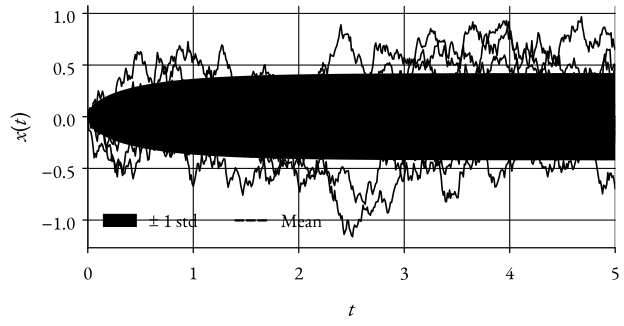
Figure 3: Ornstein-Uhlenbeck ProcessConsider the SDE,
d x ( t ) = − λ x ( t ) d t + σ d β ( t ) , x ( 0 ) = 0 , dx(t) = -\lambda x(t) \, dt + \sigma \, d\beta(t), \quad x(0) = 0, d x ( t ) = − λ x ( t ) d t + σ d β ( t ) , x ( 0 ) = 0 , where λ > 0 \lambda > 0 λ > 0 β \beta β σ \sigma σ
We have (from our previous derivation),
E [ f ( x , t ) ] = − λ E [ x ( t ) ] = − λ m ( t ) , E [ f ( x ) ( x − m ( t ) ) ] = E [ − λ x ( t ) ( x − m ( t ) ) ] = − λ E [ ( x − m ( t ) ) 2 ] = − λ p ( t ) . \begin{align*}
\mathbb{E}[f(x, t)] & = -\lambda \mathbb{E}[x(t)] = -\lambda m(t), \newline
\mathbb{E}[f(x)(x - m(t))] & = \mathbb{E}[-\lambda x(t)(x - m(t))] = -\lambda \mathbb{E}[(x - m(t))^2] = -\lambda p(t).
\end{align*} E [ f ( x , t )] E [ f ( x ) ( x − m ( t ))] = − λ E [ x ( t )] = − λm ( t ) , = E [ − λ x ( t ) ( x − m ( t ))] = − λ E [( x − m ( t ) ) 2 ] = − λ p ( t ) . This results in the ODEs,
d m ( t ) d t = − λ m ( t ) , m ( 0 ) = 0 , d p ( t ) d t = − 2 λ p ( t ) + σ 2 , p ( 0 ) = 0. \begin{align*}
\frac{d m(t)}{dt} & = -\lambda m(t), \quad m(0) = 0, \newline
\frac{d p(t)}{dt} & = -2 \lambda p(t) + \sigma^2, \quad p(0) = 0.
\end{align*} d t d m ( t ) d t d p ( t ) = − λm ( t ) , m ( 0 ) = 0 , = − 2 λ p ( t ) + σ 2 , p ( 0 ) = 0. As the solution x ( t ) x(t) x ( t )
In summary, the mean and covariance are governed by,
d m d t = E [ f ( x , t ) ] , d P d t = E [ ( x − m ( t ) ) f T ] + E [ f ( x , t ) ( x − m ( t ) ) T ] + E [ L ( x , t ) L T ( x , t ) ] . \begin{align*}
\frac{d \mathbf{m}}{dt} & = \mathbb{E}\left[\mathbf{f}(\mathbf{x}, t) \right], \newline
\frac{d \mathbf{P}}{dt} & = \mathbb{E}\left[(\mathbf{x} - \mathbf{m}(t)) \mathbf{f}^T\right] + \mathbb{E}\left[\mathbf{f}(\mathbf{x}, t) (\mathbf{x} - \mathbf{m}(t))^T\right] + \mathbb{E}\left[\mathbf{L}(\mathbf{x}, t) \mathbf{L}^T(\mathbf{x}, t)\right].
\end{align*} d t d m d t d P = E [ f ( x , t ) ] , = E [ ( x − m ( t )) f T ] + E [ f ( x , t ) ( x − m ( t ) ) T ] + E [ L ( x , t ) L T ( x , t ) ] . Note that the expectations are with respect to the density p ( x , t ) p(\mathbf{x}, t) p ( x , t )
To solve these ODEs, in general, we need to know p ( x , t ) p(\mathbf{x}, t) p ( x , t )
In the linear-Gaussian case, the first two moments characterize the solution.
Backward Kolmogorov Equation
Let the transition probability function be denoted,
p ( x ( τ ) ∣ x ( t ) ) = p x ( τ ) ∣ x ( t ) ( y , τ ; x , t ) = p ( y , τ ∣ x , t ) with τ ≥ t . p(x(\tau) \mid x(t)) = p_{x(\tau) \mid x(t)}(y, \tau; x, t) = p(y, \tau \mid x, t) \text{ with } \tau \geq t. p ( x ( τ ) ∣ x ( t )) = p x ( τ ) ∣ x ( t ) ( y , τ ; x , t ) = p ( y , τ ∣ x , t ) with τ ≥ t . Then, one can similarly derive the Kolmogorov backward equation ,
Definition 3 (Definition: Kolmogorov backward equation) − ∂ p ( y , τ ; x , t ) ∂ τ = f ( y , τ ) ∂ p ( y , τ ; x , t ) ∂ y + 1 2 L ( y , τ ) 2 ∂ 2 p ( y , τ ; x , t ) ∂ y 2 . -\frac{\partial p(y, \tau; x, t)}{\partial \tau} = f(y, \tau) \frac{\partial p(y, \tau; x, t)}{\partial y} + \frac{1}{2} L(y, \tau)^2 \frac{\partial^2 p(y, \tau; x, t)}{\partial y^2}. − ∂ τ ∂ p ( y , τ ; x , t ) = f ( y , τ ) ∂ y ∂ p ( y , τ ; x , t ) + 2 1 L ( y , τ ) 2 ∂ y 2 ∂ 2 p ( y , τ ; x , t ) . If the end conditions are known for some T , p ( x , T ) T, p(x, T) T , p ( x , T ) T T T
This is the key to generative modeling via de-noising diffusion processes 1
Consider the Itô process,
d x ( t ) = f ( x ( t ) , t ) d t + L ( x ( t ) , t ) d β ( t ) . dx(t) = f(x(t), t) \, dt + L(x(t), t) \, d\beta(t). d x ( t ) = f ( x ( t ) , t ) d t + L ( x ( t ) , t ) d β ( t ) . Then, there exists a reverse Itô process of the form 2
d x ( t ) = f ˉ ( x ( t ) , t ) d t + L ˉ ( x ( t ) , t ) d β ˉ ( t ) , dx(t) = \bar{f}(x(t), t) \, dt + \bar{L}(x(t), t) \, d\bar{\beta}(t), d x ( t ) = f ˉ ( x ( t ) , t ) d t + L ˉ ( x ( t ) , t ) d β ˉ ( t ) , defined in some region t ≤ T t \leq T t ≤ T
x ( T ) x(T) x ( T ) β ˉ \bar{\beta} β ˉ
x ( T ) − x ( t ) = ∫ t T f ˉ ( x ( s ) , s ) d s + ∫ t T L ˉ ( x ( s ) , s ) d β ˉ ( s ) . x(T) - x(t) = \int_{t}^{T} \bar{f}(x(s), s) \, ds + \int_{t}^{T} \bar{L}(x(s), s) \, d\bar{\beta}(s). x ( T ) − x ( t ) = ∫ t T f ˉ ( x ( s ) , s ) d s + ∫ t T L ˉ ( x ( s ) , s ) d β ˉ ( s ) . Lastly, consider the Itô process of the probabilistic de-noising diffusion model,
d x ( t ) = f ( x ( t ) , t ) d t + σ ( t ) d β ( t ) . d\mathbf{x}(t) = \mathbf{f}(\mathbf{x}(t), t) \, dt + \sigma(t) \, d\beta(t). d x ( t ) = f ( x ( t ) , t ) d t + σ ( t ) d β ( t ) . Then, the reverse Itô process is given by 2
d x ( t ) = [ f ( x ( t ) , t ) − σ ( t ) 2 ∇ x log p ( x ( t ) , t ) ] d t + σ ( t ) d β ˉ ( t ) . d\mathbf{x}(t) = \left[\mathbf{f}(\mathbf{x}(t), t) - \sigma(t)^2 \nabla_{\mathbf{x}} \log p(\mathbf{x}(t), t)\right] dt + \sigma(t) \, d\bar{\beta}(t). d x ( t ) = [ f ( x ( t ) , t ) − σ ( t ) 2 ∇ x log p ( x ( t ) , t ) ] d t + σ ( t ) d β ˉ ( t ) . The quantity,
∇ x log p ( x ( t ) , t ) \nabla_{\mathbf{x}} \log p(\mathbf{x}(t), t) ∇ x log p ( x ( t ) , t ) is known as the score function and is the basis for score-based generative models .
Summary
The probability density function p ( x , t ) p(x, t) p ( x , t ) Fokker-Planck-Kolmogorov equation .
There are two forms of the Fokker-Planck-Kolmogorov equation,
Forward Kolmogorov equation (Fokker-Planck equation) — evolves the density forward in time.Backward Kolmogorov equation — evolves transition probabilities backward in time.
The mean m ( t ) m(t) m ( t ) covariance p ( t ) p(t) p ( t ) p ( x , t ) p(x, t) p ( x , t )
In linear-Gaussian cases, the mean and covariance are sufficient — they fully determine the solution.
These tools are foundational for diffusion-based generative models , filtering theory, and stochastic control.