Introduction
In this part we’ll introduce Doob’s h h h
Recall our definition of the SDE,
d x ( t ) = f ( x ( t ) , t ) d t ⏟ drift + L ( x ( t ) , t ) d β ( t ) ⏟ diffusion , dx(t) = \underbrace{f(x(t), t) \, dt}_{\text{drift}} + \underbrace{L(x(t), t) \, d\beta(t)}_{\text{diffusion}}, d x ( t ) = drift f ( x ( t ) , t ) d t + diffusion L ( x ( t ) , t ) d β ( t ) , By the end of this, we’ll have a tool in our toolbox to transform this SDE into a new SDE with the following form,
and we’ll already propose that,
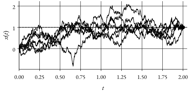
d x ( t ) = v − x ( t ) T − t d t + d β ( t ) , t ≤ T , dx(t) = \frac{v - x(t)}{T - t} dt + d\beta(t), t \leq T, d x ( t ) = T − t v − x ( t ) d t + d β ( t ) , t ≤ T , is already a special case of Equation (1) . For clarity, we read the above SDE as, as we move towards time T T T v v v
So, essentially, we’re taking a Brownian motion and forcing it to a point v v v T T T
Figure 1: Brownian motion forced to a pointRecap: Density and Bayes’ Rule
Let’s firstly recap what we know about densities and Bayes’ rule.
If we have a random value x x x x x x p x p_x p x
P ( x ∈ A ) = ∫ A p x ( x ) d x , P(x \in A) = \int_A p_x(x) \, dx, P ( x ∈ A ) = ∫ A p x ( x ) d x , or in a sloppier notation,
p x ( x ) = P ( x ∈ A ) d x . p_x(x) = \frac{P(x \in A)}{dx}. p x ( x ) = d x P ( x ∈ A ) . We say ( x , y ) (x,y) ( x , y ) p x , y p_{x,y} p x , y
P ( x ∈ A , y ∈ B ) = ∫ A ∫ B p x , y ( x , y ) d y d x , P(x \in A, y \in B) = \int_A \int_B p_{x,y}(x,y) \, dy \, dx, P ( x ∈ A , y ∈ B ) = ∫ A ∫ B p x , y ( x , y ) d y d x , Further, Bayes’ rule states that,
P ( A ∣ B ) = P ( A ∩ B ) P ( B ) . P(A \mid B) = \frac{P(A \cap B)}{P(B)}. P ( A ∣ B ) = P ( B ) P ( A ∩ B ) . We say that ( x , y ) (x,y) ( x , y ) conditional density p y ∣ x p_{y \mid x} p y ∣ x
P ( y ∈ A ∣ x ∈ B ) = P x , y ( x , y ) p x ( x ) = p x , y ( x , y ) ∫ p x , y ( x , y ) d y , P(y \in A \mid x \in B) = \frac{P_{x, y}(x, y)}{p_x(x)} = \frac{p_{x,y}(x,y)}{\int p_{x, y}(x, y) dy}, P ( y ∈ A ∣ x ∈ B ) = p x ( x ) P x , y ( x , y ) = ∫ p x , y ( x , y ) d y p x , y ( x , y ) , where we in the second step used marginalization to get the denominator.
One can also write Bayes’ rule in terms of conditionals,
P ( A ∣ B ) = P ( A ) P ( B ∣ A ) P ( B ) , P(A \mid B) = \frac{P(A) P(B \mid A)}{P(B)}, P ( A ∣ B ) = P ( B ) P ( A ) P ( B ∣ A ) , or in terms of densities,
P ( x ∈ A ∣ y ∈ B ) = p x ( x ) p y ∣ x ( y ∣ x ) p y ( y ) . P(x \in A \mid y \in B) = \frac{p_x(x) p_{y \mid x}(y \mid x)}{p_y(y)}. P ( x ∈ A ∣ y ∈ B ) = p y ( y ) p x ( x ) p y ∣ x ( y ∣ x ) . Transition Density
Now, let’s try to formulate what we’ll call transition density .
If x ( t ) x(t) x ( t ) t ≥ 0 t \geq 0 t ≥ 0 Markov process 1
p ( x ( t ) ∣ x ( s ) ) = P ( x ( t ) ∈ d y ∣ x ( s ) = x ) d y ∣ y = x ( t ) x = x ( s ) p(x(t) \mid x(s)) = \frac{P(x(t) \in dy \mid x(s) = x)}{dy} \biggr\rvert_{\substack{y = x(t) \newline x = x(s)}} p ( x ( t ) ∣ x ( s )) = d y P ( x ( t ) ∈ d y ∣ x ( s ) = x ) y = x ( t ) x = x ( s ) or in words, the conditional density of x ( t ) x(t) x ( t ) x ( s ) = x x(s) = x x ( s ) = x
Now, think of this in the general case, since it is Markov, we now that,
P ( x ( t 0 ) , x ( t 1 ) , … , x ( t n ) ) , joint of n random variables = P ( x ( t 0 ) ) P ( x ( t 1 ) ∣ x ( t 0 ) ) … P ( x ( t n ) ∣ x ( t n − 1 ) ) . \begin{align*}
& P(x(t_0), x(t_1), \ldots, x(t_n)), \text{ joint of } n \text{ random variables} \newline
& = P(x(t_0)) P(x(t_1) \mid x(t_0)) \ldots P(x(t_n) \mid x(t_{n-1})).
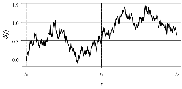
\end{align*} P ( x ( t 0 ) , x ( t 1 ) , … , x ( t n )) , joint of n random variables = P ( x ( t 0 )) P ( x ( t 1 ) ∣ x ( t 0 )) … P ( x ( t n ) ∣ x ( t n − 1 )) . Figure 2: Brownian “bridges”Champan-Kolmogorov
We’ll make use of a equation called Chapman-Kolmogorov equation 2
P ( x ( t ) ∣ x ( s ) ) = ∫ P ( x ( t ) ∣ x ( u ) ) P ( x ( u ) ∣ x ( s ) ) d x ( u ) , s < u < t , P(x(t) \mid x(s)) = \int P(x(t) \mid x(u)) P(x(u) \mid x(s)) \, dx(u), \quad s < u < t, P ( x ( t ) ∣ x ( s )) = ∫ P ( x ( t ) ∣ x ( u )) P ( x ( u ) ∣ x ( s )) d x ( u ) , s < u < t , We will not prove or further discuss this equation, but it is important to know that it exists.
Example: Transition Density of a Brownian Motion
Let’s now try to apply what we’ve learned so far to a Brownian motion.
Tip (Example: Transition density of a Brownian motion) So, we have,
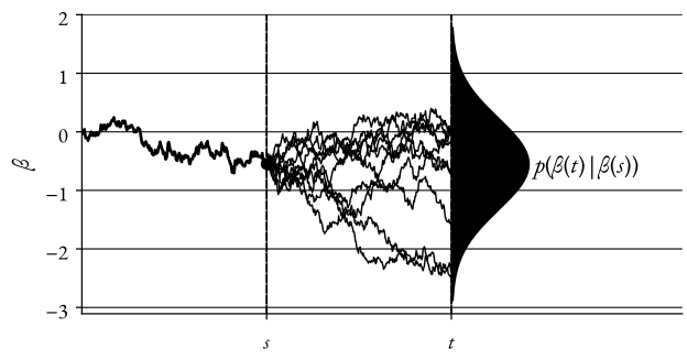
P ( β ( t ) ∣ β ( s ) ) = 1 2 π ( t − s ) exp ( − ( β ( t ) − β ( s ) ) 2 2 ( t − s ) ) , P(\beta(t) \mid \beta(s)) = \frac{1}{\sqrt{2 \pi (t - s)}} \exp\left(-\frac{(\beta(t) - \beta(s))^2}{2(t - s)}\right), P ( β ( t ) ∣ β ( s )) = 2 π ( t − s ) 1 exp ( − 2 ( t − s ) ( β ( t ) − β ( s ) ) 2 ) , and if we visualize this.
Figure 3: Transition density of a Brownian motionLet’s first start with an example and see how we can solve it.
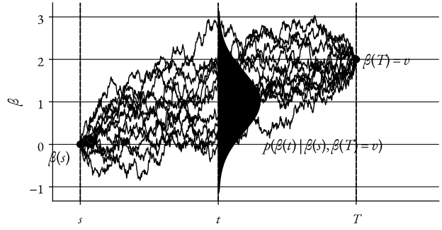
Tip (Example: Doob’s h h h What is the transition density of β ( ⋅ ) \beta(\cdot) β ( ⋅ ) β ( T ) = v \beta(T) = v β ( T ) = v transition density with p ⋆ p^\star p ⋆
p ⋆ ( β ( t ) ∣ β ( s ) ) = P ( β ( t ) ∈ d y ∣ β ( s ) = x , β ( T ) = v ) d y ∣ y = β ( t ) p^\star(\beta(t) \mid \beta(s)) = \frac{P(\beta(t) \in dy \mid \beta(s) = x, \beta(T) = v)}{dy} \biggr\rvert_{y = \beta(t)} p ⋆ ( β ( t ) ∣ β ( s )) = d y P ( β ( t ) ∈ d y ∣ β ( s ) = x , β ( T ) = v ) y = β ( t ) Which we can write as,
= P ( β ( s ) ) P ( β ( t ) ∣ β ( s ) ) h ( β ( t ) , t ) ∫ P ( β ( s ) ) P ( β ( t ) ∣ β ( s ) ) h ( β ( t ) , t ) d β ( t ) , \begin{equation}
= \frac{P(\beta(s)) P(\beta(t) \mid \beta(s)) h(\beta(t), t)}{\int P(\beta(s)) P(\beta(t) \mid \beta(s)) h(\beta(t), t) d \beta(t)},
\end{equation} = ∫ P ( β ( s )) P ( β ( t ) ∣ β ( s )) h ( β ( t ) , t ) d β ( t ) P ( β ( s )) P ( β ( t ) ∣ β ( s )) h ( β ( t ) , t ) , where
h ( s , x ) = P ( β ( T ) ∈ d y ∣ β ( s ) = x ) d y ∣ y = v h(s, x) = \frac{P(\beta(T) \in dy \mid \beta(s) = x)}{dy} \biggr\rvert_{y = v} h ( s , x ) = d y P ( β ( T ) ∈ d y ∣ β ( s ) = x ) y = v Figure 4: Transition density of a Brownian “bridge”Now, you may already see that, if h ( s , x ) h(s, x) h ( s , x ) ∇ log h ( s , x ) ⟹ v − x T − s \nabla \log h(s, x) \implies \frac{v - x}{T - s} ∇ log h ( s , x ) ⟹ T − s v − x
By the Chapman-Kolmogorov equation, we can write,
P ( β ( t ) ∣ β ( s ) ) h ( β ( t ) , t ) h ( β ( s ) , s ) , \frac{P(\beta(t) \mid \beta(s)) h(\beta(t), t)}{h(\beta(s), s)}, h ( β ( s ) , s ) P ( β ( t ) ∣ β ( s )) h ( β ( t ) , t ) , which is precisely what we’ll call Doob’s h h h .
Infinitesimal generator
Imagine we have an arbitrary function g g g
g ↦ f ⋅ g ′ + 1 2 L 2 ⋅ g ′ ′ , g \mapsto f \cdot g^\prime + \frac{1}{2} L^2 \cdot g^{\prime \prime}, g ↦ f ⋅ g ′ + 2 1 L 2 ⋅ g ′′ , or in full notation,
g ( x ) ↦ f ( x ) ⋅ g ′ ( x ) + 1 2 L 2 ( x ) ⋅ g ′ ′ ( x ) , g(x) \mapsto f(x) \cdot g^{\prime}(x) + \frac{1}{2} L^2(x) \cdot g^{\prime \prime}(x), g ( x ) ↦ f ( x ) ⋅ g ′ ( x ) + 2 1 L 2 ( x ) ⋅ g ′′ ( x ) , We’ll call this mapping/operator A g Ag A g
The operator A A A x ( t ) , t ≥ 0 x(t), t \geq 0 x ( t ) , t ≥ 0 f f f L L L
Let’s write down Itô’s formula with A A A
Informally,
[ E [ g ( x ) ∣ x ( s ) = x ] − g ( x ) ] t − s → t → s ( A g ) ( x ) , \frac{\left[ \mathbb{E}\left[ g(x) \mid x(s) = x \right] - g(x) \right] }{t - s} \xrightarrow{t \to s} (Ag)(x), t − s [ E [ g ( x ) ∣ x ( s ) = x ] − g ( x ) ] t → s ( A g ) ( x ) , note that E [ g ( x ) ∣ x ( s ) = x ] = g ( x ) \mathbb{E}[g(x) \mid x(s) = x] = g(x) E [ g ( x ) ∣ x ( s ) = x ] = g ( x )
Danger (Remark) Note that h ( β ( s ) , s ) h(\beta(s), s) h ( β ( s ) , s ) 3
h ( β ( s ) , s ) = ∫ P ( β ( t ) ∣ β ( s ) ) h ( β ( t ) , t ) d β ( t ) , h(\beta(s), s) = \int P(\beta(t) \mid \beta(s)) h(\beta(t), t) d \beta(t), h ( β ( s ) , s ) = ∫ P ( β ( t ) ∣ β ( s )) h ( β ( t ) , t ) d β ( t ) , or in other words, the drift term in Itô’s formula disappears.
Hence, ( A g ) ( x ) + ∂ ∂ s h ( s , x ) = 0 (Ag)(x) + \frac{\partial}{\partial s} h(s, x) = 0 ( A g ) ( x ) + ∂ s ∂ h ( s , x ) = 0
So, h h h backward Kolmogorov equation !
Recall that Equation (2) holds for x ( t ) x(t) x ( t )
d x ( t ) = f ( x ( t ) , t ) d t ⏟ drift + L ( x ( t ) , t ) d β ( t ) ⏟ diffusion , dx(t) = \underbrace{f(x(t), t) \, dt}_{\text{drift}} + \underbrace{L(x(t), t) \, d\beta(t)}_{\text{diffusion}}, d x ( t ) = drift f ( x ( t ) , t ) d t + diffusion L ( x ( t ) , t ) d β ( t ) , where β ( s ) \beta(s) β ( s ) x ( s ) x(s) x ( s )
Time derivative of A A A
Idea: Compute the time derivative of the conditional expectation,
E [ g ( x ( t ) ) ∣ x ( s ) = x , x ( T ) = v ] , \mathbb{E}[g(x(t)) \mid x(s) = x, x(T) = v], E [ g ( x ( t )) ∣ x ( s ) = x , x ( T ) = v ] , We’ll call the new A A A A ⋆ A^\star A ⋆
( ∂ ∂ s g + A ⋆ g ) ( x ) = lim t → s E [ g ( x ( t ) ) ∣ x ( s ) = x , x ( T ) = v ] − g ( x ) t − s = lim t → s E [ g ( x ( t ) ) − g ( x ( s ) ) ∣ x ( s ) = x , x ( T ) = v ] t − s = lim t → s ∫ g ( x ( t ) ) − g ( x ( s ) ) p ⋆ ( x ( t ) ∣ x ( s ) ) d x ( t ) = lim t → s ∫ [ g ( x ( t ) ) − g ( x ( s ) ) ] h ( x ( t ) , t ) h ( x ( s ) , s ) p ( x ( t ) ∣ x ( s ) ) d x ( t ) = lim t → s E [ [ g ( x ( t ) ) − g ( x ( s ) ) ] h ( x ( t ) , t ) ∣ x ( s ) = x ] h ( x ( s ) , s ) = 1 h ( s , x ) ( ( ∂ ∂ s + A ) ( h g ) ) ( s , x ) . \begin{align*}
(\frac{\partial}{\partial s} g + A^\star g)(x) & = \lim_{t \to s} \frac{\mathbb{E}[g(x(t)) \mid x(s) = x, x(T) = v] - g(x)}{t - s} \newline
& = \lim_{t \to s} \frac{\mathbb{E}[g(x(t)) - g(x(s)) \mid x(s) = x, x(T) = v]}{t - s} \newline
& = \lim_{t \to s} \int g(x(t)) - g(x(s)) p^\star(x(t) \mid x(s)) \, dx(t) \newline
& = \lim_{t \to s} \int \left[ g(x(t)) - g(x(s)) \right] \frac{h(x(t), t)}{h(x(s), s)} p(x(t) \mid x(s)) \, dx(t) \newline
& = \lim_{t \to s} \frac{\mathbb{E}[[g(x(t)) - g(x(s))] h(x(t), t) \mid x(s) = x]}{h(x(s), s)} \newline
& = \frac{1}{h(s, x)} \left( \left( \frac{\partial}{\partial s} + A \right) (h g) \right)(s, x).
\end{align*} ( ∂ s ∂ g + A ⋆ g ) ( x ) = t → s lim t − s E [ g ( x ( t )) ∣ x ( s ) = x , x ( T ) = v ] − g ( x ) = t → s lim t − s E [ g ( x ( t )) − g ( x ( s )) ∣ x ( s ) = x , x ( T ) = v ] = t → s lim ∫ g ( x ( t )) − g ( x ( s )) p ⋆ ( x ( t ) ∣ x ( s )) d x ( t ) = t → s lim ∫ [ g ( x ( t )) − g ( x ( s )) ] h ( x ( s ) , s ) h ( x ( t ) , t ) p ( x ( t ) ∣ x ( s )) d x ( t ) = t → s lim h ( x ( s ) , s ) E [[ g ( x ( t )) − g ( x ( s ))] h ( x ( t ) , t ) ∣ x ( s ) = x ] = h ( s , x ) 1 ( ( ∂ s ∂ + A ) ( h g ) ) ( s , x ) . This holds in general for Markov processes.
Thus, we have,
A ⋆ g = 1 h A ( h g ) = … = A g + L 2 ∇ h h ⋅ g ′ = ( f + L 2 ∇ log h ) g ′ + 1 2 L 2 g ′ ′ \begin{align*}
A^\star g & = \frac{1}{h} A(h g) = \ldots = Ag + L^2 \frac{\nabla h}{h} \cdot g^\prime \newline
& = (f + L^2 \nabla \log h) g^\prime + \frac{1}{2} L^2 g^{\prime \prime}
\end{align*} A ⋆ g = h 1 A ( h g ) = … = A g + L 2 h ∇ h ⋅ g ′ = ( f + L 2 ∇ log h ) g ′ + 2 1 L 2 g ′′ The h h h f + L 2 ∇ log h f + L^2 \nabla \log h f + L 2 ∇ log h L 2 L^2 L 2
Girsanov’s theorem
Girsanov’s theorem states that, if we have a process x ( t ) x(t) x ( t ) f f f L L L h h h x ⋆ ( t ) x^\star(t) x ⋆ ( t )
d x ⋆ ( t ) = f ( x ⋆ ( t ) , t ) d t + L 2 ( x ⋆ ( t ) , t ) ∇ log h ( x ⋆ ( t ) , t ) d t + L ( x ⋆ ( t ) , t ) d β ( t ) , dx^\star(t) = f(x^\star(t), t) \, dt + L^2(x^\star(t), t) \nabla \log h(x^\star(t), t) \, dt + L(x^\star(t), t) \, d\beta(t), d x ⋆ ( t ) = f ( x ⋆ ( t ) , t ) d t + L 2 ( x ⋆ ( t ) , t ) ∇ log h ( x ⋆ ( t ) , t ) d t + L ( x ⋆ ( t ) , t ) d β ( t ) , and the original process x ( t ) x(t) x ( t )
d x ( t ) = f ( x ( t ) , t ) d t + L ( x ( t ) , t ) d β ( t ) , dx(t) = f(x(t), t) \, dt + L(x(t), t) \, d\beta(t), d x ( t ) = f ( x ( t ) , t ) d t + L ( x ( t ) , t ) d β ( t ) , Further, L a w ( x ⋆ ( t ) ) \mathrm{Law}(x^\star(t)) Law ( x ⋆ ( t ))
∫ P ( x ( 0 ) ) P ( x ( t ) ∣ x ( 0 ) ) h ( x ( t ) , t ) h ( x ( 0 ) , 0 ) d x ( 0 ) , \int \frac{P(x(0)) P(x(t) \mid x(0)) h(x(t), t)}{h(x(0), 0)} \, dx(0), ∫ h ( x ( 0 ) , 0 ) P ( x ( 0 )) P ( x ( t ) ∣ x ( 0 )) h ( x ( t ) , t ) d x ( 0 ) , Let’s say now that, if we choose a smart h h h x ⋆ ( t ) x^\star(t) x ⋆ ( t )
∫ P ( x ( 0 ) ) P ( x ( t ) ∣ x ( 0 ) ) h ( x ( t ) , t ) h ( x ( 0 ) , 0 ) d x ( 0 ) = π ( x ( t ) ) . \int \frac{P(x(0)) P(x(t) \mid x(0)) h(x(t), t)}{h(x(0), 0)} \, dx(0) = \pi(x(t)). ∫ h ( x ( 0 ) , 0 ) P ( x ( 0 )) P ( x ( t ) ∣ x ( 0 )) h ( x ( t ) , t ) d x ( 0 ) = π ( x ( t )) . That is what we’ll do in the next part ;).
Also, note that L a w ( x ( t ) ) \mathrm{Law}(x(t)) Law ( x ( t ))
∫ P ( x ( 0 ) ) P ( x ( t ) ∣ x ( 0 ) ) d x ( 0 ) . \int P(x(0)) P(x(t) \mid x(0)) \, dx(0). ∫ P ( x ( 0 )) P ( x ( t ) ∣ x ( 0 )) d x ( 0 ) .