Part 7 - Operator Theory and Connection to Generative (Diffusion) Models

Introduction

In this part we’ll discuss a bit of operator theory, but in general this part is to connect what we’ve seen in the last part to the overall family of generative (diffusion) models.

Recap from Lecture 6

As always, recall our definition of the SDE,

dx(t) = \underbrace{f(x(t), t) \ dt}_{\text{drift}} + \underbrace{L(x(t), t) \ d\beta(t)}_{\text{diffusion}}.

We defined the $h$ -transform as,

h(x(s), s) p(x(T) | x(s)) \biggr\vert_{\substack{x(T) = v \in \mathbb{R} \newline x(s) \in \mathbb{R}}}.

Which has an important property, namely,

\int p(x(T) | x(s)) h(x(t), t) dx(t) = h(x(s), s),

a martingale property.

We also defined the transition density,

p^{\star}(x(t) | x(s)) = \frac{p(x(t) | x(s)) h(x(t), t)}{h(x(s), s)},

which in fact uses the $h$ -transform.

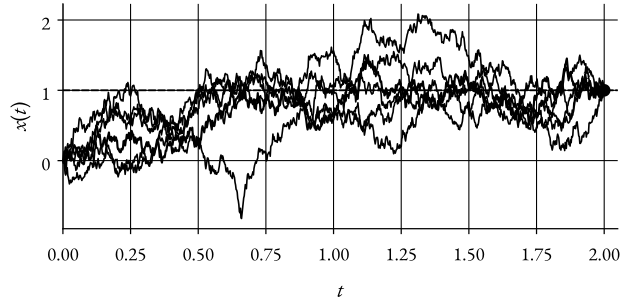
Further, we saw how the conditional process took use of the $h$ -transform (bridge to $v$ at time $T$ ),

\begin{equation} dx(t) = f(x(t), t) \ dt + L^2(x(t), t) \nabla \log h(x(t), t) \ dt + L(x(t), t) d \beta(t). \end{equation}

Brownian motion forced to a point at time

Then we defined the $A$ operator,

g(x) \mapsto (Ag)(x) = f(x) g^{\prime}(x) + \frac{1}{2} L^2(x) g^{\prime\prime}(x),

If $g(s, x)$ depends on time and state/space,

\frac{\partial}{\partial s} g(s, x) + (Ag)(s, x) = 0.

An Important Definition and Observation

Now, take $h_T(x)$ and define,

h(s, x) = \int p(x(T) | x(s)) h_T(x(T)) \ dx(T),

Here, we can make an important observation, namely,

\begin{align*} \int p(x(t) | x(s)) h(x(t), t) \ dx(t) & = \int p(x(t) | x(s)) \left( \int p(x(T) | x(s)) h_T(x(T)) d x(T) \right) d x(t) \newline & \overset{\text{C.K}}{=} \int p(x(T) | x(s)) h_T(x(T)) d x(T). \end{align*}

For each $h_T(x)$ we get a process like in Equation (1), with transition density $p^{\star}(x(t) | x(s))$ .

If $x(0) = x_0 \in \mathbb{R}$ (deterministically), then $x^{\star}(T)$ has density,

p^{\star}(x(T) | x(0)) = \frac{p(x(T) | x(0)) h_T(x(T))}{h(x(0), 0)}

Thus, if we want to sample from a density $\pi(x(T))$ ,

\begin{align*} \frac{p(x(T) | x(0)) h_T(x(T))}{h(x(0), 0)} & = \pi(x(T)) \newline h_T(x(T)) & = C \cdot \frac{\pi(x(T))}{p(x(T) | x(0))} \end{align*}

so, if you give me the data density $\pi(x(T))$ , we can obtain $h(s, x)$ (or the smarter choice is $\nabla \log h(s, x)$ , but we’ll come to this.)

Remark 1

Note that our generative model runs forward in time here, one can also reverse the time.

Example 1

$x(t)$ is a Brownian motion,

dx(t) = \underbrace{0 \ dt}_{f} + \underbrace{1 \ d\beta(t)}_{L}, \quad x(0) = 0.

Assume that $\pi$ is given, and our end time is $T = 1$ . Thus,

\begin{align*} h(x(1)) & = C \cdot \frac{\pi(x(1))}{p(x(1) | x(0))} \newline & = \tilde{C} \cdot \frac{\pi(x(1))}{e^{-\frac{x(1))^2}{2}}} \end{align*}

Which means the $h$ -transform is,

\begin{align*} h(s, x) & = \tilde{C} \int p(x(1) | x(s)) \frac{\pi(x(1))}{e^{-\frac{x(1)^2}{2}}} \ dx(1) \newline & = \tilde{\tilde{C}} \int e^{-\frac{1}{2} \frac{(x(1) - x(s))^2}{1 - s} + \frac{x(1)^2}{2}} \pi(x(1)) \ dx(1) \newline \end{align*}

Which we can write as an expectation,

= \tilde{\tilde{C}} \cdot \mathbb{E} \left[ e^{-\frac{1}{2} \frac{(x(1) - x(s))^2}{1 - s} + \frac{x(1)^2}{2}} \right].

This is useful if we don’t have $\pi$ , but have samples, $x_1 \sim \mathcal{D}$ .

Note

If $x(t)$ is a Brownian motion and $\pi(x(T))$ is given, then,

\nabla \log h(x(s), s) = \ldots = \mathbb{E}_{x(T) \sim p^{x(T) | x(s)}} \left[ \frac{x(T) - x(s)}{T - s} \right],

seems familiar? ;)

Score Matching

Recall that the “score” is defined as,

s(x(t), t) = \nabla_x \log h(x(t), t).

Note

If we take the integral over the $h$ -transformed process,

\int h(x(t), t) \ dx(t) \neq 1,

but instead,

\int h(x(t), t) \ dx(t) = C \in \mathbb{R}.

Thus, the $h$ -transform is not a probability, but likelihood [^1]. Which means, that if we normalize the $h$ -transform, we get a probability density function,

\frac{h(x(t), t)}{\int h(u, t) d u}.

Score matching learns the score from (weighted) samples of,

q(x) = \frac{h(x(t), t)}{\int h(u, t) d u}

Vanilla score matching (Hyvärinen, 2005) ¹,

Take nueral netowrk approximation, $\hat{s}_{\theta}(x(t), t) \approx s(x(t), t)$ .
Train with,

\underset{\theta}{\min} \int_0^T \int q(x(t), t) \sum_{i = 0}^d S_i \ dx(t) dt, \quad x \in \mathbb{R}^d,

where $S_i = \frac{\partial}{\partial x_i} s_{\theta}(x(t), t)^{(i)} + \frac{1}{2} s_{\theta}(x(t), t)^2$ .

Or in the scalar case,

\underset{\theta}{\min} \int_0^T \int q(x(t), t) \left(s_{\theta}^{\prime}(x(t), t) + \frac{1}{2} s_{\theta}(x(t), t)^2 \right) \ dx(t) dt,

and again, if we only have samples,

\underset{\theta}{\min} \ C \cdot \sum_K \sum_L s_{\theta}^{\prime}(x_{K, L}, t_K) + s_{\theta}(x_{K, L}, t_K)^2,

where $x_{K, L}$ are samples from $q(t_K, \cdot)$ and $C = 1, \ldots, N$ .

So, we need samples from,

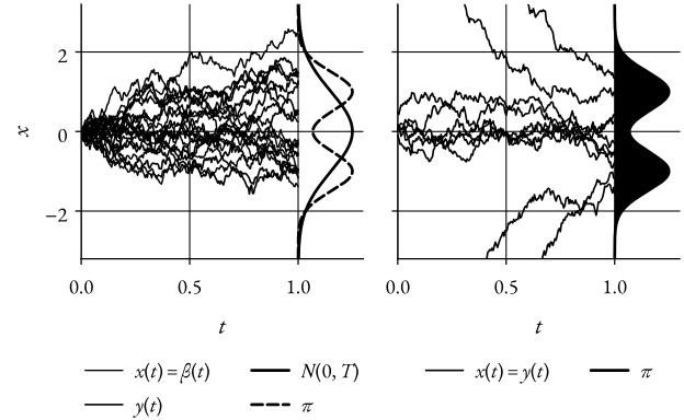
q(x(t), t) = \frac{h(x(t), t)}{\int h(u, t) d u}.

Luckily, Schoenmakers et al. (2013) ² propose,

\begin{cases} \begin{align*} dy(t) & = \alpha(y(t), t) \ dt + L(y(t)) \ d \beta(t) & \text{-- position} \newline d \mathfrak{y}(t) & = C(y(t), t) \mathfrak{y}(t) \ dt & \text{-- weights} \end{align*} \end{cases}

We have two choices for setting up stuff,

\begin{align*} \mathfrak{y}(0) & = 1 \newline y(0) & \sim \frac{h_0(x(T))}{\int h_0(v) d v} \end{align*}

\begin{align*} y(0) & \sim \pi_1 \newline \mathfrak{y}(0) & = \frac{1}{p(x(T) | x(0))} \biggr\vert_{x(T) = y(0)} \end{align*}

But the important part is that,

\begin{align*} \alpha(T - t, x) & = -f(x(t), t) + (L^2)^{\prime}(x(t), t) \newline C(T - t, x) & = \frac{1}{2} (L^2)^{\prime\prime}(x(t), t) - f^{\prime\prime}(x(t), t) \end{align*}

Example 2

For each test function $g$ ,

\mathbb{E}[g(y(t) \cdot \mathfrak{y}(t)) = \int g(x) q(t, x) \ dx.

Take $x(0) = 0, x(t) = \beta(t)$ ,

\begin{cases} \begin{align*} f & = 0 \newline L & = 1 \end{align*} \end{cases} \implies \begin{cases} \begin{align*} dy(t) & = d \beta(t), \quad \mathfrak{y}(t) = 1 \newline L^{\prime} & = L^{\prime\prime} = 0 \end{align*} \end{cases}

Score matching diffusion!

Part 7 - Operator Theory and Connection to Generative (Diffusion) Models

Introduction

Recap from Lecture 6

An Important Definition and Observation

Score Matching

Footnotes