Part 2 - Convexity I

Outline

In this part, we will cover the following topics:

  • Convex sets
  • Polytopes
  • Polyhedra
  • Cones

We will start by defining what makes a set convex.

Convex Sets

Definition 1 (Convex Set)

A set SRnS \subseteq \mathbb{R}^n is called convex if,

λx1+(1λ)x2S{(x1,x2)Sλ(0,1)\lambda \mathbf{x}_1 + (1 - \lambda) \mathbf{x}_2 \in S \begin{cases} \forall (\mathbf{x}_1, \mathbf{x}_2) \in S \newline \lambda \in (0,1) \end{cases}
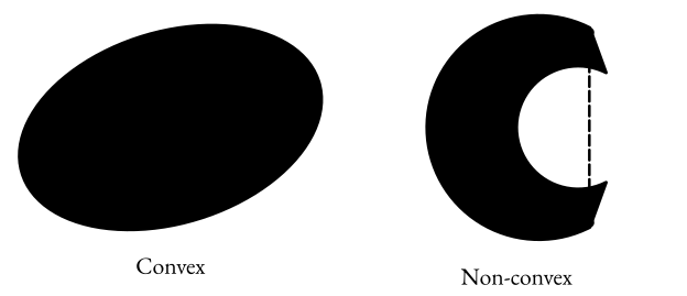
Example of a convex set and non-convex set

Examples

By definition, \emptyset is convex.

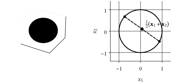
The set {xRnxa}\{\mathbf{x} \in \mathbb{R}^n \mid \Vert \mathbf{x} \Vert \leq a \} is convex aR\forall a \in \mathbb{R}.

However, the set {xRnx=a}\{\mathbf{x} \in \mathbb{R}^n \mid \Vert \mathbf{x} \Vert = a \} is not convex for any a>0a > 0.

Example of a convex set and non-convex set
Proposition 1 (Convex Set Intersection)

Let SkRnS_k \in \mathbb{R}^n for k=1,,Kk = 1, \ldots, K be convex.

Then, the intersection,

Sk=1KSk  is convex.S \coloneqq \bigcap_{k=1}^K S_k \ \text{ is convex.}
Proof

Let x1,x2S\mathbf{x}_1, \mathbf{x}_2 \in S and λ(0,1)\lambda \in (0,1). Since x1,x2S\mathbf{x}_1, \mathbf{x}_2 \in S, we have that x1,x2Sk\mathbf{x}_1, \mathbf{x}_2 \in S_k for all k=1,,Kk = 1, \ldots, K. Each SkS_k is convex, thus,

λx1+(1λ)x2Sk, k=1,,K\lambda \mathbf{x}_1 + (1 - \lambda) \mathbf{x}_2 \in S_k, \ \forall k = 1, \ldots, K

Hence, λx1+(1λ)x2\lambda \mathbf{x}_1 + (1 - \lambda) \mathbf{x}_2 lies in all the SkS_k simultaneously, i.e.,

λx1+(1λ)x2S=k=1KSk \lambda \mathbf{x}_1 + (1 - \lambda) \mathbf{x}_2 \in S = \bigcap_{k=1}^K S_k \ _\blacksquare
Note

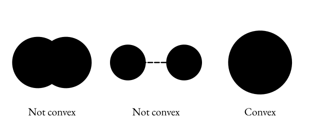
Unions of convex sets might not be convex.

Examples of the union of convex sets

Convex Hull

Definition 2 (Convex Hull)

The convex hull of a finite set of points, {v1,,vk}Rn\{\mathbf{v}_1, \ldots, \mathbf{v}_k \} \subseteq \mathbb{R}^n is defined as,

conv V{λ1v1++λkvkλ1,,λk0i=1kλi=1}\mathrm{conv} \ V \coloneqq \{\lambda_1 \mathbf{v}_1 + \ldots + \lambda_k \mathbf{v}_k \mid \lambda_1, \ldots, \lambda_k \geq 0 \sum_{i=1}^k \lambda_i = 1 \}
Definition 3 (Properties of the Convex Hull)

The convex hull of the set SRnS \subseteq \mathbb{R}^n, is the set with any of the following properties,

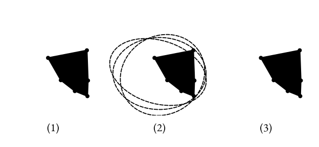
  • (1) It is the unique minimal convex set containing SS.
  • (2) It is the intersection of all convex sets containing SS.
  • (3) It is the set of all convex combinations of points in SS.
Construction of the convex hull

From (3), any point in the convex hull can be expressed as a convex combination of points in SS.

An interesting question is how many points do we need to construct the convex hull?

Theorem 1 (Carathéodory’s Theorem)

Let αconv(S)\alpha \in \mathrm{conv}(S), where SRnS \subseteq \mathbb{R}^n.

Then α\alpha can be expressed as a convex combination of at most n+1n+1 points in SS.

Polytopes

Definition 4 (Polytope)

A set PRnP \subseteq \mathbb{R}^n is called a polytope if it is the convex hull of finitely many points.

Note

A polytope will always have straight edges. So, a circle is not a polytope (since the circumference is curved and can not be expressed with finitely many points).

Definition 5 (Extreme Point)

A point v\mathbf{v} of a convex set SS is called an extreme point if,

v=x1=x2{v=λx1+(1λ)x2x1,x2Sλ(0,1)\mathbf{v} = \mathbf{x}_1 = \mathbf{x}_2 \begin{cases} \mathbf{v} = \lambda \mathbf{x}_1 + (1 - \lambda) \mathbf{x}_2 \newline \mathbf{x}_1, \mathbf{x}_2 \in S \newline \lambda \in (0,1) \end{cases}
Theorem 2 (Extreme Points of a Polytope)

Let PP be the polytope conv(V)\mathrm{conv}(V), where V={v1,,vk}V = \{\mathbf{v}_1, \ldots, \mathbf{v}_k \}. Then, PP is equal to the convex hull of its extreme points.

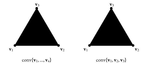
Extreme points of different polytopes

Polyhedra

Definition 6 (Polyhedron)

A set PP is called a polyhedron if there exists a matrix ARn×mA \in \mathbb{R}^{n \times m} and a vector bRn\mathbf{b} \in \mathbb{R}^n such that,

P{xRmAxb}P \coloneqq \{\mathbf{x} \in \mathbb{R}^m \mid A\mathbf{x} \leq \mathbf{b} \}
Note

AxbA\mathbf{x} \leq \mathbf{b} means that,

aiTxbi, i=1,,n\mathbf{a}_i^T \mathbf{x} \leq b_i, \ \forall i = 1, \ldots, n

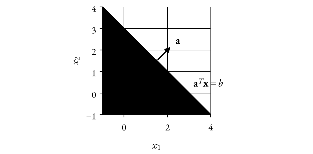
where aiT\mathbf{a}_i^T is the ii-th row of AA and bib_i is the ii-th element of b\mathbf{b}. Further, {xRmAxb}\{\mathbf{x} \in \mathbb{R}^m \mid A\mathbf{x} \leq \mathbf{b} \} is a half-space. A polyhedron is the intersection of nn half-spaces     \implies a polyhedron is a convex set (by our previous proposition).

Half-space defined by a linear inequality
Example 1 (Polyhedron)

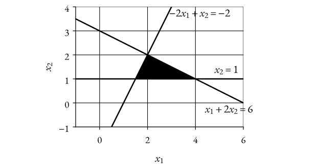
Let A=[122101]A = \begin{bmatrix} 1 & 2 \newline -2 & 1 \newline 0 & -1 \end{bmatrix} and b=[621]\mathbf{b} = \begin{bmatrix} 6 \newline -2 \newline -1 \end{bmatrix}. This gives the following system of inequalities,

{x1+2x262x1+x22x21\begin{cases} x_1 + 2x_2 \leq 6 \newline -2x_1 + x_2 \leq -2 \newline -x_2 \leq -1 \end{cases}
Polyhedron defined by the intersection of half-spaces
Theorem 3 (Extreme Points of a Polyhedron)

Let xP{xRmAxb}\mathbf{x}^{\prime} \in P \{\mathbf{x} \in \mathbb{R}^m \mid A\mathbf{x} \leq \mathbf{b} \}, where ARn×mA \in \mathbb{R}^{n \times m}, rank(A)=m\mathrm{rank}(A) = m and bRn\mathbf{b} \in \mathbb{R}^n.

Further, let Ax=bA^{\prime} \mathbf{x}^{\prime} = \mathbf{b}^{\prime} be the equality subsystem of AxbA\mathbf{x} \leq \mathbf{b}, i.e., A\mathbf{A}^{\prime} contains all rows of AA where we have (Ax)i=bi(A \mathbf{x}^{\prime})_i = b_i.

Then, x\mathbf{x}^{\prime} is an extreme point of PP if and only if rank(A)=m\mathrm{rank}(A^{\prime}) = m.

Example 2 (Continued)

Let x=[321]\mathbf{x}^{\prime} = \begin{bmatrix} \frac{3}{2} \newline 1 \end{bmatrix}. Then,

Ax=[7221],b=[621]Axb    [7221][621]\begin{align*} A \mathbf{x}^{\prime} & = \begin{bmatrix} \frac{7}{2} \newline -2 \newline -1 \end{bmatrix}, \mathbf{b} = \begin{bmatrix} 6 \newline -2 \newline -1 \end{bmatrix} \newline A \mathbf{x}^{\prime} \leq \mathbf{b} & \implies \begin{bmatrix} \frac{7}{2} \newline -2 \newline -1 \end{bmatrix} \leq \begin{bmatrix} 6 \newline -2 \newline -1 \end{bmatrix} \end{align*}

Which means,

A=[2101],b=[21]\mathbf{A}^{\prime} = \begin{bmatrix} -2 & 1 \newline 0 & -1 \end{bmatrix}, \mathbf{b}^{\prime} = \begin{bmatrix} -2 \newline -1 \end{bmatrix}

We can see that rank(A)=2=m\mathrm{rank}(\mathbf{A}^{\prime}) = 2 = m, thus x\mathbf{x}^{\prime} is an extreme point of PP.

Example 3 (Continued)

Now, consider a new point x2=[21]\mathbf{x}^{\prime}_2 = \begin{bmatrix} 2 \newline 1 \end{bmatrix}. Then,

Ax2=[431]Ax2b    [431][621]\begin{align*} A \mathbf{x}^{\prime}_2 & = \begin{bmatrix} 4 \newline -3 \newline -1 \end{bmatrix} \newline A \mathbf{x}^{\prime}_2 \leq \mathbf{b} & \implies \begin{bmatrix} 4 \newline -3 \newline -1 \end{bmatrix} \leq \begin{bmatrix} 6 \newline -2 \newline -1 \end{bmatrix} \end{align*}

Which means,

A2=[01],b2=[1]\mathbf{A}^{\prime}_2 = \begin{bmatrix} 0 & -1 \end{bmatrix}, \mathbf{b}^{\prime}_2 = \begin{bmatrix} -1 \end{bmatrix}

We can see that rank(A2)=1m\mathrm{rank}(\mathbf{A}^{\prime}_2) = 1 \neq m, thus x2\mathbf{x}^{\prime}_2 is not an extreme point of PP.

Cones

Definition 7 (Cone)

A set CRnC \subseteq \mathbb{R}^n is a cone if,

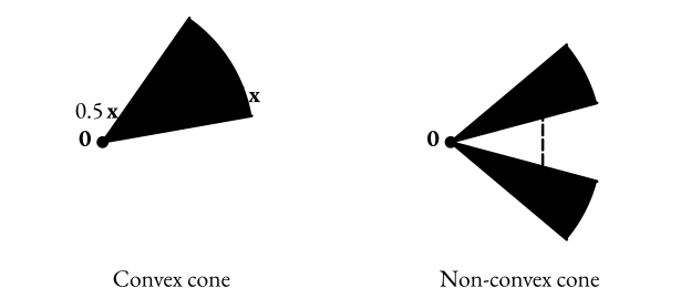
λxC, xC, λ>0\lambda \mathbf{x} \in C, \ \forall \mathbf{x} \in C, \ \lambda > 0
Examples of cones
Examples of cones
Example 4 (Convex Cone)

Let ARn×mA \subseteq \mathbb{R}^{n \times m} then, C{xRmAx0}C \coloneqq \{\mathbf{x} \in \mathbb{R}^m \mid A\mathbf{x} \leq 0 \} is a convex cone.

It is quite simple to prove this, assume that xC\mathbf{x} \in C and λ>0\lambda > 0,

A(λx)=λ>0Ax00 A(\lambda \mathbf{x}) = \underbrace{\underbrace{\lambda}_{> 0} \underbrace{A\mathbf{x}}_{\leq 0}}_{\leq 0} \ _\blacksquare

Representation Theorem

Theorem 4 (Representation Theorem)

Let Q={xRmAxb}Q = \{\mathbf{x} \in \mathbb{R}^m \mid A\mathbf{x} \leq \mathbf{b} \} (polyhedron) and let {v1,,vk}\{\mathbf{v}_1, \ldots, \mathbf{v}_k \} be its extreme points. Further, we define Pconv({v1,,vk})P \coloneqq \mathrm{conv}(\{\mathbf{v}_1, \ldots, \mathbf{v}_k \}) (polytope) and C{xRmAx0}C \coloneqq \{\mathbf{x} \in \mathbb{R}^m \mid A\mathbf{x} \leq 0 \} (cone). Then,

Q=P+C={xRmx=u+v, uP, vC}\begin{align*} Q & = P + C \newline & = \{\mathbf{x} \in \mathbb{R}^m \mid \mathbf{x} = \mathbf{u} + \mathbf{v}, \ \mathbf{u} \in P, \ \mathbf{v} \in C \} \end{align*}
Corollary 1 (Bounded Polyhedron)

A bounded polyhedron is a polytope.

Let’s state the pros and cons of polytopes and polyhedra.

  • Polytope
    • Pros: Easy to get extreme points (by definition).
    • Cons: Hard to check if new point is inside.
  • Polyhedron
    • Pros: Easy to check if new point is inside.
    • Cons: Hard to get extreme points (need to check intersection of half-spaces, grows combinatorially, infeasible for large problems).