Outline
In this part, we will cover the following topics:
Convex functions
The epigraph of a function
Characterizations of convex functions
Subgradients & subdifferentials
Convex optimization problems
We will start by defining convex functions and exploring their properties.
Convex Functions
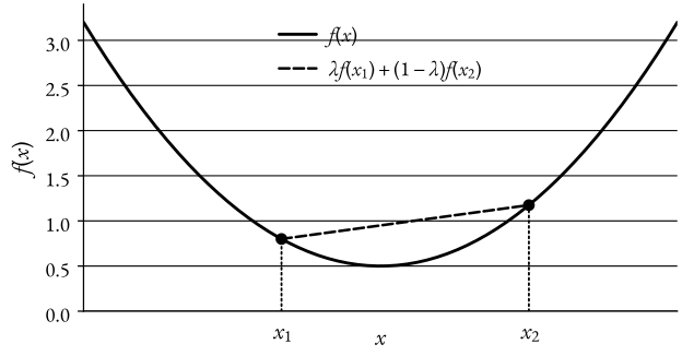
Definition 1 (Convex Function) Suppose S ⊆ R n S \subseteq \mathbb{R}^n S ⊆ R n is a convex set. Let f : S ↦ R f: S \mapsto \mathbb{R} f : S ↦ R be a function.
We say that f f f is a convex function if,
f ( λ x 1 + ( 1 − λ ) x 2 ) ≤ λ f ( x 1 ) + ( 1 − λ ) f ( x 2 ) { ∀ x 1 , x 2 ∈ S , λ ∈ ( 0 , 1 ) f(\lambda \mathbf{x}_1 + (1-\lambda) \mathbf{x}_2) \leq \lambda f(\mathbf{x}_1) + (1-\lambda) f(\mathbf{x}_2)
\begin{cases}
\forall \mathbf{x}_1, \mathbf{x}_2 \in S, \newline
\lambda \in (0,1)
\end{cases} f ( λ x 1 + ( 1 − λ ) x 2 ) ≤ λ f ( x 1 ) + ( 1 − λ ) f ( x 2 ) { ∀ x 1 , x 2 ∈ S , λ ∈ ( 0 , 1 )
Convex Function Definition
Note It is called strictly convex if the inequality is strict for x 1 ≠ x 2 \mathbf{x}_1 \neq \mathbf{x}_2 x 1 = x 2 , i.e.,
f ( λ x 1 + ( 1 − λ ) x 2 ) < λ f ( x 1 ) + ( 1 − λ ) f ( x 2 ) { ∀ x 1 , x 2 ∈ S , λ ∈ ( 0 , 1 ) , x 1 ≠ x 2 f(\lambda \mathbf{x}_1 + (1-\lambda) \mathbf{x}_2) < \lambda f(\mathbf{x}_1) + (1-\lambda) f(\mathbf{x}_2)
\begin{cases}
\forall \mathbf{x}_1, \mathbf{x}_2 \in S, \newline
\lambda \in (0,1), \newline
\mathbf{x}_1 \neq \mathbf{x}_2
\end{cases} f ( λ x 1 + ( 1 − λ ) x 2 ) < λ f ( x 1 ) + ( 1 − λ ) f ( x 2 ) ⎩ ⎨ ⎧ ∀ x 1 , x 2 ∈ S , λ ∈ ( 0 , 1 ) , x 1 = x 2
The function is called concave if − f -f − f is convex.
Example 1 (Some Convex Functions) f ( x ) = c T x + d , c ∈ R n , d ∈ R , f(\mathbf{x}) = \mathbf{c}^T \mathbf{x} + d, \quad \mathbf{c} \in \mathbb{R}^n, d \in \mathbb{R}, f ( x ) = c T x + d , c ∈ R n , d ∈ R , is both convex and concave (only function that is both convex and concave).
f ( x ) = ∥ x ∥ f(\mathbf{x}) = \Vert \mathbf{x} \Vert f ( x ) = ∥ x ∥ is convex.
f ( x ) = ∥ x ∥ 2 f(\mathbf{x}) = \Vert \mathbf{x} \Vert^2 f ( x ) = ∥ x ∥ 2 is strictly convex.
Proposition 1 (Non-negative Weighted Sum of Convex Functions is Convex) Let S ⊆ R n S \subseteq \mathbb{R}^n S ⊆ R n be a convex set and f k : S ↦ R , k = 1 , … , K f_k: S \mapsto \mathbb{R}, k=1, \ldots, K f k : S ↦ R , k = 1 , … , K be convex functions.
Let α k ≥ 0 , k = 1 , … , K \alpha_k \geq 0, k=1, \ldots, K α k ≥ 0 , k = 1 , … , K . Then,
f ( x ) ≔ ∑ k = 1 K α k f k ( x ) is convex. f(\mathbf{x}) \coloneqq \sum_{k=1}^K \alpha_k f_k(\mathbf{x}) \ \text{is convex.} f ( x ) : = k = 1 ∑ K α k f k ( x ) is convex.
Proposition 2 (Composition of Convex Functions) Let g : R n ↦ R g: \mathbb{R}^n \mapsto \mathbb{R} g : R n ↦ R be a convex function and f : R ↦ R f: \mathbb{R} \mapsto \mathbb{R} f : R ↦ R 1 1 Note that one can generalize this statement, the domains do not necessarily need to be R n \mathbb{R}^n R n and R \mathbb{R} R , respectievly. be a convex function and non-decreasing 2 2 The motivation here is, if we have f ( x ) = − x f(x) = -x f ( x ) = − x , our composition will become concave. function. Then, the composition f ( g ( x ) ) f(g(\mathbf{x})) f ( g ( x )) is convex.
Example 2 (Composition of Convex Functions) Let f( x ) = e x (x) = e^x ( x ) = e x and g ( x ) = x 2 g(x) = x^2 g ( x ) = x 2 . Both are convex on R \mathbb{R} R and f f f is non-decreasing.
By our proposition, f ( g ( x ) ) = e x 2 f(g(x)) = e^{x^2} f ( g ( x )) = e x 2 is convex (on R \mathbb{R} R ) 3 3 Note that if we restrict our domain to R + \mathbb{R}^{+} R + , g ( x ) = x 2 g(x) = x^2 g ( x ) = x 2 becomes non-decreasing and thus g ( f ( x ) ) = ( e x ) 2 = e 2 x g(f(x)) = (e^x)^2 = e^{2x} g ( f ( x )) = ( e x ) 2 = e 2 x is convex on R + \mathbb{R}^{+} R + as well. .
The Epigraph of a Function
Definition 2 (Epigraph of a Function) The epigraph of a function f : R n ↦ R ∪ { ± ∞ } f: \mathbb{R}^n \mapsto \mathbb{R} \cup \{\pm \infty \} f : R n ↦ R ∪ { ± ∞ } is defined as,
e p i ( f ) ≔ { ( x , α ) ∈ R n × R ∣ f ( x ) ≤ α } \mathrm{epi}(f) \coloneqq \{(\mathbf{x}, \alpha) \in \mathbb{R}^n \times \mathbb{R} \mid f(\mathbf{x}) \leq \alpha \} epi ( f ) : = {( x , α ) ∈ R n × R ∣ f ( x ) ≤ α }
Note e p i ( f ) ⊆ R n + 1 \mathrm{epi}(f) \subseteq \mathbb{R}^{n+1} epi ( f ) ⊆ R n + 1
Theorem 1 (Characterization of Convex Functions via Epigraphs) f f f is convex if and only if e p i ( f ) \mathrm{epi}(f) epi ( f ) is a convex set.]
Definition 3 (C 1 C^1 C 1 Functions) C 1 ≔ set of all continuously differentiable functions C^1 \coloneqq \text{set of all continuously differentiable functions} C 1 : = set of all continuously differentiable functions
Characterizations of Convexity (of C 1 C^1 C 1 Functions)
Theorem 2 (First Order Characterization of Convexity) Let f ∈ C 1 f \in C^1 f ∈ C 1 on an open convext set S S S . Then,
f is convex ⟺ f ( x ) ≥ f ( x ′ ) + ∇ f ( x ′ ) T ( x − x ′ ) , ∀ x , x ′ ∈ S f \text{ is convex} \iff f(\mathbf{x}) \geq f(\mathbf{x^{\prime}}) + \nabla f(\mathbf{x^{\prime}})^T (\mathbf{x} - \mathbf{x^{\prime}}), \quad \forall \mathbf{x}, \mathbf{x^{\prime}} \in S f is convex ⟺ f ( x ) ≥ f ( x ′ ) + ∇ f ( x ′ ) T ( x − x ′ ) , ∀ x , x ′ ∈ S
Proof (First Order Characterization of Convexity) Let f f f be a convex functrion. Let x , x ′ ∈ S \mathbf{x}, \mathbf{x^{\prime}} \in S x , x ′ ∈ S and λ ∈ ( 0 , 1 ) \lambda \in (0,1) λ ∈ ( 0 , 1 ) . By the definition of convexity,
f ( λ x + ( 1 − λ ) x ′ ) ≤ λ f ( x ) + ( 1 − λ ) f ( x ′ ) ⏟ f ( x ′ ) − λ f ( x ′ ) f ( x ) − f ( x ′ ) ≥ f ( λ x + ( 1 − λ ) x ′ ) − f ( x ′ ) λ ≥ f ( x ′ + λ ( x − x ′ ) ) − f ( x ′ ) λ \begin{align*}
f(\lambda \mathbf{x} + (1-\lambda) \mathbf{x^{\prime}}) & \leq \lambda f(\mathbf{x}) + \underbrace{(1-\lambda) f(\mathbf{x^{\prime}})}_{f(\mathbf{x}^{\prime}) - \lambda f(\mathbf{x}^{\prime})} \newline
f(\mathbf{x}) - f(\mathbf{x^{\prime}}) & \geq \frac{f(\lambda \mathbf{x} + (1-\lambda) \mathbf{x^{\prime}}) - f(\mathbf{x^{\prime}})}{\lambda} \newline
& \geq \frac{f(\mathbf{x^{\prime}} + \lambda (\mathbf{x} - \mathbf{x^{\prime}})) - f(\mathbf{x^{\prime}})}{\lambda} \newline
\end{align*} f ( λ x + ( 1 − λ ) x ′ ) f ( x ) − f ( x ′ ) ≤ λ f ( x ) + f ( x ′ ) − λ f ( x ′ ) ( 1 − λ ) f ( x ′ ) ≥ λ f ( λ x + ( 1 − λ ) x ′ ) − f ( x ′ ) ≥ λ f ( x ′ + λ ( x − x ′ )) − f ( x ′ ) If we now let λ → 0 + \lambda \to 0^{+} λ → 0 + , we get,
f ( x ) − f ( x ′ ) ≥ ∇ f ( x ′ ) T ( x − x ′ ) f ( x ) ≥ f ( x ′ ) + ∇ f ( x ′ ) T ( x − x ′ ) ■ \begin{align*}
f(\mathbf{x}) - f(\mathbf{x^{\prime}}) & \geq \nabla f(\mathbf{x^{\prime}})^T (\mathbf{x} - \mathbf{x^{\prime}}) \newline
f(\mathbf{x}) & \geq f(\mathbf{x^{\prime}}) + \nabla f(\mathbf{x^{\prime}})^T (\mathbf{x} - \mathbf{x^{\prime}}) \ _\blacksquare
\end{align*} f ( x ) − f ( x ′ ) f ( x ) ≥ ∇ f ( x ′ ) T ( x − x ′ ) ≥ f ( x ′ ) + ∇ f ( x ′ ) T ( x − x ′ ) ■ Now, let,
f ( x ) ≥ f ( x ′ ) + ∇ f ( x ′ ) T ( x − x ′ ) , ∀ x , x ′ ∈ S f(\mathbf{x}) \geq f(\mathbf{x^{\prime}}) + \nabla f(\mathbf{x^{\prime}})^T (\mathbf{x} - \mathbf{x^{\prime}}), \quad \forall \mathbf{x}, \mathbf{x^{\prime}} \in S f ( x ) ≥ f ( x ′ ) + ∇ f ( x ′ ) T ( x − x ′ ) , ∀ x , x ′ ∈ S Let x 1 , x 2 ∈ S \mathbf{x}_1, \mathbf{x}_2 \in S x 1 , x 2 ∈ S and λ ∈ ( 0 , 1 ) \lambda \in (0,1) λ ∈ ( 0 , 1 ) . We set x = x 1 \mathbf{x} = \mathbf{x}_1 x = x 1 and x ′ = λ x 1 + ( 1 − λ ) x 2 \mathbf{x^{\prime}} = \lambda \mathbf{x}_1 + (1-\lambda) \mathbf{x}_2 x ′ = λ x 1 + ( 1 − λ ) x 2 in the above inequality to get,
f ( x 1 ) ≥ f ( λ x 1 + ( 1 − λ ) x 2 ) + ∇ f ( λ x 1 + ( 1 − λ ) x 2 ) T ( x 1 − ( λ x 1 + ( 1 − λ ) x 2 ) ) f(\mathbf{x}_1) \geq f(\lambda \mathbf{x}_1 + (1-\lambda) \mathbf{x}_2) + \nabla f(\lambda \mathbf{x}_1 + (1-\lambda) \mathbf{x}_2)^T (\mathbf{x}_1 - (\lambda \mathbf{x}_1 + (1-\lambda) \mathbf{x}_2)) f ( x 1 ) ≥ f ( λ x 1 + ( 1 − λ ) x 2 ) + ∇ f ( λ x 1 + ( 1 − λ ) x 2 ) T ( x 1 − ( λ x 1 + ( 1 − λ ) x 2 )) Further, we set x = x 2 \mathbf{x} = \mathbf{x}_2 x = x 2 and x ′ = λ x 1 + ( 1 − λ ) x 2 \mathbf{x^{\prime}} = \lambda \mathbf{x}_1 + (1-\lambda) \mathbf{x}_2 x ′ = λ x 1 + ( 1 − λ ) x 2 in the above inequality to get,
f ( x 2 ) ≥ f ( λ x 1 + ( 1 − λ ) x 2 ) + ∇ f ( λ x 1 + ( 1 − λ ) x 2 ) T ( x 2 − ( λ x 1 + ( 1 − λ ) x 2 ) ) f(\mathbf{x}_2) \geq f(\lambda \mathbf{x}_1 + (1-\lambda) \mathbf{x}_2) + \nabla f(\lambda \mathbf{x}_1 + (1-\lambda) \mathbf{x}_2)^T (\mathbf{x}_2 - (\lambda \mathbf{x}_1 + (1-\lambda) \mathbf{x}_2)) f ( x 2 ) ≥ f ( λ x 1 + ( 1 − λ ) x 2 ) + ∇ f ( λ x 1 + ( 1 − λ ) x 2 ) T ( x 2 − ( λ x 1 + ( 1 − λ ) x 2 )) Multiplying the first inequality by λ \lambda λ and the second by ( 1 − λ ) (1-\lambda) ( 1 − λ ) and adding them, we get,
λ f ( x 1 ) + ( 1 − λ ) f ( x 2 ) ≥ f ( λ x 1 + ( 1 − λ ) x 2 ) + ∇ f ( λ x 1 + ( 1 − λ ) x 2 ) T ( λ ( x 1 − ( λ x 1 + ( 1 − λ ) x 2 ) ) + ( 1 − λ ) ( x 2 − ( λ x 1 + ( 1 − λ ) x 2 ) ) ) = f ( λ x 1 + ( 1 − λ ) x 2 ) + ∇ f ( λ x 1 + ( 1 − λ ) x 2 ) T ⋅ 0 = f ( λ x 1 + ( 1 − λ ) x 2 ) ■ \begin{align*}
\lambda f(\mathbf{x}_1) + (1-\lambda) f(\mathbf{x}_2) & \geq f(\lambda \mathbf{x}_1 + (1-\lambda) \mathbf{x}_2) + \nabla f(\lambda \mathbf{x}_1 + (1-\lambda) \mathbf{x}_2)^T \newline
& \quad (\lambda (\mathbf{x}_1 - (\lambda \mathbf{x}_1 + (1-\lambda) \mathbf{x}_2)) + (1-\lambda) (\mathbf{x}_2 - (\lambda \mathbf{x}_1 + (1-\lambda) \mathbf{x}_2))) \newline
& = f(\lambda \mathbf{x}_1 + (1-\lambda) \mathbf{x}_2) + \nabla f(\lambda \mathbf{x}_1 + (1-\lambda) \mathbf{x}_2)^T \cdot 0 \newline
& = f(\lambda \mathbf{x}_1 + (1-\lambda) \mathbf{x}_2) \ _\blacksquare
\end{align*} λ f ( x 1 ) + ( 1 − λ ) f ( x 2 ) ≥ f ( λ x 1 + ( 1 − λ ) x 2 ) + ∇ f ( λ x 1 + ( 1 − λ ) x 2 ) T ( λ ( x 1 − ( λ x 1 + ( 1 − λ ) x 2 )) + ( 1 − λ ) ( x 2 − ( λ x 1 + ( 1 − λ ) x 2 ))) = f ( λ x 1 + ( 1 − λ ) x 2 ) + ∇ f ( λ x 1 + ( 1 − λ ) x 2 ) T ⋅ 0 = f ( λ x 1 + ( 1 − λ ) x 2 ) ■
Subgradients & Subdifferentials
Definition 4 (Subgradient) Let S ⊆ R n S \subseteq \mathbb{R}^n S ⊆ R n be a convex set and f : S ↦ R f: S \mapsto \mathbb{R} f : S ↦ R be a convex function.
P ∈ R n P \in \mathbb{R}^n P ∈ R n is called a subgradient of f f f at x ′ ∈ S \mathbf{x^{\prime}} \in S x ′ ∈ S if,
f ( x ) ≥ f ( x ′ ) + P T ( x − x ′ ) , ∀ x ∈ S f(\mathbf{x}) \geq f(\mathbf{x^{\prime}}) + P^T (\mathbf{x} - \mathbf{x^{\prime}}), \quad \forall \mathbf{x} \in S f ( x ) ≥ f ( x ′ ) + P T ( x − x ′ ) , ∀ x ∈ S
Definition 5 (Subdifferential) Let S ⊆ R n S \subseteq \mathbb{R}^n S ⊆ R n be a convex set and f : S ↦ R f: S \mapsto \mathbb{R} f : S ↦ R be a convex function. The subdifferential of f f f at x ′ ∈ S \mathbf{x^{\prime}} \in S x ′ ∈ S is defined as,
∂ f ( x ′ ) ≔ { P ∈ R n ∣ f ( x ) ≥ f ( x ′ ) + P T ( x − x ′ ) , ∀ x ∈ S } \partial f(\mathbf{x^{\prime}}) \coloneqq \{ P \in \mathbb{R}^n \mid f(\mathbf{x}) \geq f(\mathbf{x^{\prime}}) + P^T (\mathbf{x} - \mathbf{x^{\prime}}), \quad \forall \mathbf{x} \in S \} ∂ f ( x ′ ) : = { P ∈ R n ∣ f ( x ) ≥ f ( x ′ ) + P T ( x − x ′ ) , ∀ x ∈ S } Or, in other words, the set of all subgradients of f f f at x ′ \mathbf{x^{\prime}} x ′ .
Proposition 3 (Subdifferential of Differentiable Convex Function) Let S ⊆ R n S \subseteq \mathbb{R}^n S ⊆ R n be a convex set and f : S ↦ R f: S \mapsto \mathbb{R} f : S ↦ R be a convex function. If x ′ ∈ i n t S \mathbf{x}^{\prime} \in \mathrm{int} \ S x ′ ∈ int S 4 4 i n t S \mathrm{int} \ S int S is the interior of S S S . , and f f f is differentiable at x ′ \mathbf{x}^{\prime} x ′ , then,
∂ f ( x ′ ) = { ∇ f ( x ′ ) } \partial f(\mathbf{x^{\prime}}) = \{ \nabla f(\mathbf{x^{\prime}}) \} ∂ f ( x ′ ) = { ∇ f ( x ′ )}
Characterizations of Convexity (of C 2 C^2 C 2 Functions)
Theorem 3 (Second Order Characterization of Convexity) Let S ⊆ R n S \subseteq \mathbb{R}^n S ⊆ R n be an open convex set and f ∈ C 2 f \in C^2 f ∈ C 2 on S S S . Then,
f is convex ⟺ ∇ 2 f ( x ) ⪰ 0 , ∀ x ∈ S f \text{ is convex} \iff \nabla^2 f(\mathbf{x}) \succeq 0, \quad \forall \mathbf{x} \in S f is convex ⟺ ∇ 2 f ( x ) ⪰ 0 , ∀ x ∈ S where ∇ 2 f ( x ) \nabla^2 f(\mathbf{x}) ∇ 2 f ( x ) is the Hessian of f f f at x \mathbf{x} x and ⪰ 0 \succeq 0 ⪰ 0 means positive semidefinite.
Further,
∇ 2 f ( x ) ≻ 0 , ∀ x ∈ S ⟹ f is strictly convex \nabla^2 f(\mathbf{x}) \succ 0, \quad \forall \mathbf{x} \in S \implies f \text{ is strictly convex} ∇ 2 f ( x ) ≻ 0 , ∀ x ∈ S ⟹ f is strictly convex
Notice how in the second part, we only have an implication and not an equivalence. This is because the converse is not necessarily true.
Example 3 (Second Order Characterization of Convexity) Let f ( x ) = x 4 f(x) = x_4 f ( x ) = x 4 this is a strictly convex and the gradient is,
∇ f ( x ) = 4 x 3 \nabla f(x) = 4x^3 ∇ f ( x ) = 4 x 3 The Hessian is,
∇ 2 f ( x ) = 12 x 2 , \nabla^2 f(x) = 12x^2, ∇ 2 f ( x ) = 12 x 2 , But,
∇ 2 f ( 0 ) = 0 ⊁ 0 \nabla^2 f(0) = 0 \nsucc 0 ∇ 2 f ( 0 ) = 0 ⊁ 0
Example 4 (Second Order Characterization of Convexity) Let f ( x ) = 1 2 x T Q x − q T x f(\mathbf{x}) = \frac{1}{2} \mathbf{x}^T Q \mathbf{x} - \mathbf{q}^T \mathbf{x} f ( x ) = 2 1 x T Q x − q T x , where Q ∈ R n × n Q \in \mathbb{R}^{n \times n} Q ∈ R n × n is a symmetric matrix (i.e., Q = Q T Q = Q^T Q = Q T ) and q ∈ R n \mathbf{q} \in \mathbb{R}^n q ∈ R n . The gradient is,
∇ f ( x ) = Q x − q \nabla f(\mathbf{x}) = Q \mathbf{x} - \mathbf{q} ∇ f ( x ) = Q x − q The Hessian is,
∇ 2 f ( x ) = Q \nabla^2 f(\mathbf{x}) = Q ∇ 2 f ( x ) = Q Thus, by the second order characterization of convexity, f f f is convex if and only if Q ⪰ 0 Q \succeq 0 Q ⪰ 0 .
Convex Optimization Problems
Consider the problem P P P
min x f ( x ) subject to g i ( x ) ≤ 0 , i ∈ I g i ( x ) = 0 , i ∈ E x ∈ X \begin{align*}
\min_{\mathbf{x}} \ & f(\mathbf{x}) \newline
\text{subject to } & g_i(\mathbf{x}) \leq 0, \quad i \in \mathcal{I} \newline
& g_i(\mathbf{x}) = 0, \quad i \in \mathcal{E} \newline
& \mathbf{x} \in X
\end{align*} x min subject to f ( x ) g i ( x ) ≤ 0 , i ∈ I g i ( x ) = 0 , i ∈ E x ∈ X
P P P is called a convex problem if,
(1) f f f is convex,
(2) g i , i ∈ I g_i, i \in \mathcal{I} g i , i ∈ I are convex,
(3) g i , i ∈ E g_i, i \in \mathcal{E} g i , i ∈ E are affine,
(4) X X X is a convex set.
These conditions make sure that { x ∈ R n ∣ g i ( x ) ≤ 0 , i ∈ I } \{\mathbf{x} \in \mathbb{R}^n \mid g_i(\mathbf{x}) \leq 0, i \in \mathcal{I} \} { x ∈ R n ∣ g i ( x ) ≤ 0 , i ∈ I } is a convex set and { x ∈ R n ∣ g i ( x ) = 0 , i ∈ E } \{\mathbf{x} \in \mathbb{R}^n \mid g_i(\mathbf{x}) = 0, i \in \mathcal{E} \} { x ∈ R n ∣ g i ( x ) = 0 , i ∈ E } is a convext set.
Note Very, very often we will minimize a function, but sometimes maximizing a function can be more natural, but we have to be careful.
min f ( x ) ⟺ − max − f ( x ) \min \ f(\mathbf{x}) \iff -\max \ -f(\mathbf{x}) min f ( x ) ⟺ − max − f ( x ) Therefore, also max f ( x ) \max \ f(\mathbf{x}) max f ( x ) for a concave function f f f is a convex problem.