Overview

Part 11 - Calculation methods for AC-circuits

In this part we’ll cover all calculation methods that we’ll use for AC-circuits.

Equivalent Impedance

Given the circuit and that ω=5 rad/s\omega = 5 \ \mathrm{rad/s} - find the equivalent output impedance:
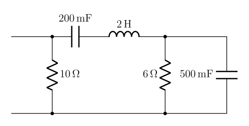
Circuit for the equivalent impedance example.
Figure 1: Circuit for the equivalent impedance example.

As we discussed in the last part, our resistor rules for series and parallel apply for impedance as well.

Let’s first quickly convert the capacitor and inductor to Ohm.

For our capacitor:

ZC=1jωC=−j⋅1ωC=−j⋅15⋅500⋅10−3 [Ω]=−j0.4 Ω.\begin{align*} Z_{C} & = \dfrac{1}{j\omega C} \newline & = -j \cdot \dfrac{1}{\omega C} \newline & = -j \cdot \dfrac{1}{5 \cdot 500 \cdot 10^{-3}} \ [\Omega] \newline & = -j0.4 \ \Omega. \end{align*}

Same procedure for our inductor:

ZL=jωL=j(5⋅2) [Ω]=j10 Ω.\begin{align*} Z_{L} & = j\omega L \newline & = j(5 \cdot 2) \ [\Omega] \newline & = j10 \ \Omega. \end{align*}

Which means we have the following circuit now:
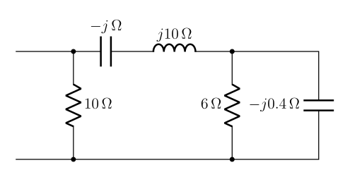
The same circuit with the impedances.
Figure 2: The same circuit with the impedances.

Now, let’s simplify our impedance!

Z6∥−j0.4=(6)(−j0.4)6−j0.4=−j2.46−j0.4=(−j2.4)(6+j0.4)(6−j0.4)(6+j0.4)=(−j2.4)(6+j0.4)36.16=0.96−j14.436.16=0.96−j14.436.16∠0∘=14.43∠−86.18∘36.16∠0∘=14.4336.16∠−86.18∘=0.399∠−86.18∘=0.026−j0.39 Ω.\begin{align*} Z_{6 \parallel -j0.4} & = \dfrac{(6)(-j0.4)}{6 - j0.4} \newline & = \dfrac{-j2.4}{6 - j0.4} \newline & = \dfrac{(-j2.4)(6 + j0.4)}{(6 - j0.4)(6 + j0.4)} \newline & = \dfrac{(-j2.4)(6 + j0.4)}{36.16} \newline & = \dfrac{0.96 - j14.4}{36.16} \newline & = \dfrac{0.96 - j14.4}{36.16 \angle 0^{\circ}} \newline & = \dfrac{14.43 \angle -86.18^{\circ}}{36.16 \angle 0^{\circ}} \newline & = \dfrac{14.43}{36.16} \angle -86.18^{\circ} \newline & = 0.399 \angle -86.18^{\circ} \newline & = 0.026 - j0.39 \ \Omega. \end{align*} Zseries=−j+j10+0.026−j0.39=0.026+j8.61 Ω.\begin{align*} Z_{\text{series}} & = -j + j10 + 0.026 - j0.39 \newline & = 0.026 + j8.61 \ \Omega. \end{align*} Z10∥0.026+j8.61=(10)(0.026+j8.61)10+0.026+j8.61=0.26+j86.110.026+j8.61=86.1∠89.82∘13.21∠40.65∘=86.113.21∠(89.82∘−40.65∘)=6.51∠49.17∘ Ω.\begin{align*} Z_{10 \parallel 0.026 + j8.61} & = \dfrac{(10)(0.026 + j8.61)}{10 + 0.026 + j8.61} \newline & = \dfrac{0.26 + j86.1}{10.026 + j8.61} \newline & = \dfrac{86.1 \angle 89.82^{\circ}}{13.21 \angle 40.65^{\circ}} \newline & = \dfrac{86.1}{13.21} \angle (89.82^{\circ} - 40.65^{\circ}) \newline & = \boxed{6.51 \angle 49.17^{\circ} \ \Omega}. \end{align*}

Multiple sources

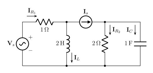
Given this circuit, and that ω=2 rad/s\omega = 2 \ \mathrm{rad/s}, Ic=2∠28∘I_{c} = 2 \angle 28^{\circ} - find IS\mathbf{I}_S and I(t)I(t).

Circuit with multiple sources.
Figure 3: Circuit with multiple sources.

Here we can utilize Ohm’s law,

Vc=IcZc=1jωCIc=−j1ωCIc=−j12(2∠28∘)=(−j0.5)(2∠28∘)=(12∠−90∘)(2∠28∘)=12⋅2∠(−90∘+28∘)=1∠−62∘.\begin{align*} V_{c} & = I_{c} Z_{c} \newline & = \dfrac{1}{j\omega C} I_{c} \newline & = -j \dfrac{1}{\omega C} I_{c} \newline & = -j \dfrac{1}{2} (2 \angle 28^{\circ}) \newline & = (-j0.5)(2 \angle 28^{\circ}) \newline & = \left(\dfrac{1}{2} \angle -90^{\circ}\right)(2 \angle 28^{\circ}) \newline & = \dfrac{1}{2} \cdot 2 \angle (-90^{\circ} + 28^{\circ}) \newline & = 1 \angle -62^{\circ}. \end{align*}

We know that VR2=VCV_{R_2} = V_{C} since they are in parallel!

IR2=VR2ZR2=VCZR2=VC2=12∠−62∘.\begin{align*} I_{R_2} & = \dfrac{V_{R_2}}{Z_{R_{2}}} \newline & = \dfrac{V_{C}}{Z_{R_{2}}} \newline & = \dfrac{V_{C}}{2} \newline & = \dfrac{1}{2} \angle -62^{\circ}. \end{align*}

Using Kirchhoff’s current law we know that,

IS=IR2+IC=(12∠−62∘)+(2∠28∘)=(0.23−j0.44)+(1.76+j0.93)=1.99+j0.49=2.04∠13.83∘.\begin{align*} \mathbf{I}_S & = I_{R_2} + I_{C} \newline & = \left(\dfrac{1}{2} \angle -62^{\circ}\right) + (2 \angle 28^{\circ}) \newline & = (0.23 - j0.44) + (1.76 + j0.93) \newline & = 1.99 + j0.49 \newline & = \boxed{2.04 \angle 13.83^{\circ}}. \end{align*}

Which means that I(t)I(t),

I(t)=2.04cos⁡(2t+13.83∘) A.\boxed{I(t) = 2.04 \cos(2t + 13.83^{\circ}) \ \mathrm{A}}.

Node Analysis

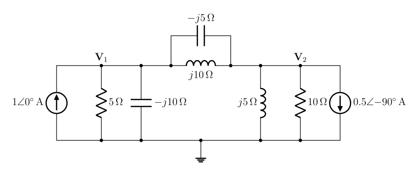
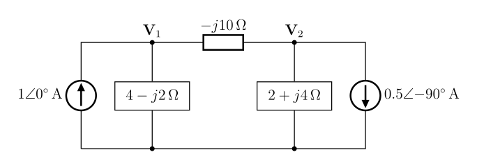
Given this circuit, find V1V_1 and V2V_2:

Circuit for node analysis.
Figure 4: Circuit for node analysis.

Let’s perform our node analysis algorithm here:

For V1V_1,

−1∠0∘+V15+V1−j10+V1−V2−j5+V1−V2j10=0V15+jV110+jV1−V25−jV1−V210=10.2V1+j0.1V1+j0.2(V1−V2)−j0.1(V1−V2)=10.2V1+j0.1V1+j0.2V1−j0.2V2−j0.1V1+j0.1V2=10.2V1+j0.2V1−j0.1V2=1(0.2+j0.2)V1−j0.1V2=1(0.2+j0.2)V1=1+j0.1V2V1=1+j0.1V20.2+j0.2.\begin{align*} & -1 \angle 0^{\circ} + \dfrac{V_1}{5} + \dfrac{V_1}{-j10} + \dfrac{V_1 - V_2}{-j5} + \dfrac{V_1 - V_2}{j10} = 0 \newline & \dfrac{V_1}{5} + j\dfrac{V_1}{10} + j\dfrac{V_1 - V_2}{5} - j\dfrac{V_1 - V_2}{10} = 1 \newline & 0.2V_1 + j0.1V_1 + j0.2(V_1 - V_2) - j0.1(V_1 - V_2) = 1 \newline & 0.2V_1 + j0.1V_1 + j0.2V_1 - j0.2V_2 -j0.1V_1 + j0.1V_2 = 1 \newline & 0.2V_1 + j0.2V_1 - j0.1V_2 = 1 \newline & (0.2 + j0.2)V_1 - j0.1V_2 = 1 \newline & (0.2 + j0.2)V_1 = 1 + j0.1V_2 \newline & V_1 = \dfrac{1 + j0.1V_2}{0.2 + j0.2}. \end{align*}

For V2V_2,

V2−V1−j5+V2−V1j10+V2j5+V210+0.5∠90∘=0jV2−V15−jV2−V110−V25+V210−j0.5=0j0.2(V2−V1)−j0.1(V2−V1)−0.2V2+0.1V2−j0.5=0j0.2V2−j0.2V1−j0.1V2+j0.1V1−0.2V2+0.1V2−j0.5=0−0.1V2+j0.1V2−j0.1V1=j0.5(0.1−j0.1)V2−j0.1V1=j0.5V2=j0.5+j0.1V10.1−j0.1.\begin{align*} & \dfrac{V_2 - V_1}{-j5} + \dfrac{V_2 - V_1}{j10} + \dfrac{V_2}{j5} + \dfrac{V_2}{10} + 0.5 \angle 90^{\circ} = 0 \newline & j\dfrac{V_2 - V_1}{5} - j\dfrac{V_2 - V_1}{10} - \dfrac{V_2}{5} + \dfrac{V_2}{10} - j0.5 = 0 \newline & j0.2(V_2 - V_1) - j0.1(V_2 - V_1) - 0.2V_2 + 0.1V_2 - j0.5 = 0 \newline & j0.2V_2 - j0.2V_1 - j0.1V_2 + j0.1V_1 - 0.2V_2 + 0.1V_2 - j0.5 = 0 \newline & -0.1V_2 + j0.1V_2 - j0.1V_1 = j0.5 \newline & (0.1 - j0.1)V_2 - j0.1V_1 = j0.5 \newline & V_2 = \dfrac{j0.5 + j0.1V_1}{0.1 - j0.1}. \end{align*}

Now finding V1V_1 and V2V_2, by substituting V1V_1 in this,

V2=…=−2+j4 V=4.47∠116.6∘ V.\begin{align*} V_2 & = \ldots = -2 + j4 \ \mathrm{V} \newline & = \boxed{4.47 \angle 116.6^{\circ} \ \mathrm{V}}. \end{align*}

Which means V2(t)V_2(t),

V2(t)=4.47cos⁡(ωt+116.6∘).V_2(t) = \boxed{4.47 \cos(\omega t + 116.6^{\circ})}.

For V1V_1,

V1=…=1−j2 V=2.24∠−63.4∘ V.\begin{align*} V_1 & = \ldots = 1 - j2 \ \mathrm{V} \newline & = \boxed{2.24 \angle -63.4^{\circ} \ \mathrm{V}}. \end{align*}

Which means V1(t)V_1(t),

V1(t)=2.24cos⁡(ωt−63.4∘).V_1(t) = \boxed{2.24 \cos(\omega t - 63.4^{\circ})}.

Mesh analysis

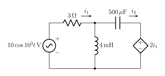
Given this circuit, find I1(t)I_1(t) and I2(t)I_2(t):

Circuit for mesh analysis.
Figure 5: Circuit for mesh analysis.

Let’s first quickly convert our capacitor and inductor:

Our inductor:

ZL=jωL=j(103⋅4⋅10−3) [Ω]=j4 Ω.\begin{align*} Z_{L} & = j\omega L \newline & = j(10^3 \cdot 4 \cdot 10^{-3}) \ [\Omega] \newline & = j4 \ \Omega. \end{align*}

Our capacitor:

ZC=−j1ωC=−j1103⋅500⋅10−6=−j2 Ω.\begin{align*} Z_{C} & = -j \dfrac{1}{\omega C} \newline & = -j \dfrac{1}{10^3 \cdot 500 \cdot 10^{-6}} \newline & = -j2 \ \Omega. \end{align*}

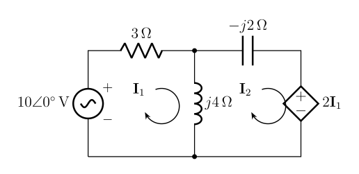
Which gives us:

The same circuit with the impedances and mesh currents.
Figure 6: The same circuit with the impedances and mesh currents.

For Mesh 1,

−10∠0∘+3I1+j4(I1−I2)=0(3+j4)I1−j4I2=10.\begin{align*} -10 \angle 0^{\circ} + 3I_1 + j4(I_1 - I_2) & = 0 \newline (3 + j4)I_1 - j4I_2 & = 10. \end{align*}

For Mesh 2,

j4(I2−I1)−j2I2+2I1=0(2−j4)I1+j2I2=0.\begin{align*} j4(I_2 - I_1) - j2I_2 + 2I_1 & = 0 \newline (2 - j4)I_1 + j2I_2 & = 0. \end{align*}

Finding I1I_1 and I2I_2,

I1=14+j813=1.24∠29.7∘ A,\begin{align*} I_1 & = \dfrac{14 + j8}{13} \newline & = \boxed{1.24 \angle 29.7^{\circ} \ \mathrm{A}}, \end{align*} I2=20+j3013=2.77∠56.3∘ A.\begin{align*} I_2 & = \dfrac{20 + j30}{13} \newline & = \boxed{2.77 \angle 56.3^{\circ} \ \mathrm{A}}. \end{align*}

Meaning that,

I1(t)=1.24cos⁡(103t+29.7∘),I2(t)=2.77cos⁡(103t+56.3∘).\begin{align*} I_1(t) & = 1.24 \cos(10^3 t + 29.7^{\circ}), \newline I_2(t) & = 2.77 \cos(10^3 t + 56.3^{\circ}). \end{align*}

Superposition

Looking at this circuit again:

Circuit for node analysis.
Figure 7: Circuit for node analysis.

One can see that we can solve this via the principle of superposition.

We first need to simplify our circuit impedance,

Z−j5∥j10=(−j5)(j10)−j5+j10=50j5=50∠0∘j5=50∠0∘5∠90∘=505∠−90∘=10∠−90∘=−j10 Ω.\begin{align*} Z_{-j5 \parallel j10} & = \dfrac{(-j5)(j10)}{-j5 + j10} \newline & = \dfrac{50}{j5} \newline & = \dfrac{50 \angle 0^{\circ}}{j5} \newline & = \dfrac{50 \angle 0^{\circ}}{5 \angle 90^{\circ}} \newline & = \dfrac{50}{5} \angle -90^{\circ} \newline & = 10 \angle -90^{\circ} \newline & = -j10 \ \Omega. \end{align*} Z5∥−j10=(5)(−j10)5−j10=(5)(−j10)(5+j10)(5−j10)(5+j10)=(−j50)(5+j10)52+102=500−j250125=4−j2 Ω.\begin{align*} Z_{5 \parallel -j10} & = \dfrac{(5)(-j10)}{5 - j10} \newline & = \dfrac{(5)(-j10)(5 + j10)}{(5 - j10)(5 + j10)} \newline & = \dfrac{(-j50)(5 + j10)}{5^2 + 10^2} \newline & = \dfrac{500 - j250}{125} \newline & = 4 - j2 \ \Omega. \end{align*} Zj5∥10=…=2+j4 Ω.\begin{align*} Z_{j5 \parallel 10} & = \ldots = 2 + j4 \ \Omega. \end{align*}

Which means:

The simplified circuit.
Figure 8: The simplified circuit.

When right source is off,

(4−j2)∥(−j10+2+j4)V1L=1∠0∘(4−j2)(−j10+2+j4)(4−j2)+(−j10+2+j4)=…=2−j2 V.\begin{align*} & (4 - j2) \parallel (-j10 + 2 + j4) \newline V_{1L} & = 1 \angle 0^{\circ} \dfrac{(4 - j2)(-j10 + 2 + j4)}{(4 - j2) + (-j10 + 2 + j4)} \newline & = \ldots \newline & = 2 - j2 \ \mathrm{V}. \end{align*}

Left source turned off,

(4−j2−j10)∥(2+j4)V1R=(−0.5∠−90∘)(2+j44−j2−j10+2+j4)(4−j2)=…=−1 V.\begin{align*} & (4 - j2 - j10) \parallel (2 + j4) \newline V_{1R} & = (-0.5 \angle -90^{\circ}) \left(\dfrac{2 + j4}{4 - j2 - j10 + 2 + j4}\right) (4 - j2) \newline & = \ldots \newline & = -1 \ \mathrm{V}. \end{align*}

Which means,

V1=V1L+V1R=2−j2−1=1−j2 V.\begin{align*} V_1 & = V_{1L} + V_{1R} \newline & = 2 - j2 - 1 \newline & = 1 - j2 \ \mathrm{V}. \end{align*}

Same procedure for V2V_2.

Thévenin equivalent

Given this circuit, find the Thévenin equivalent circuit:
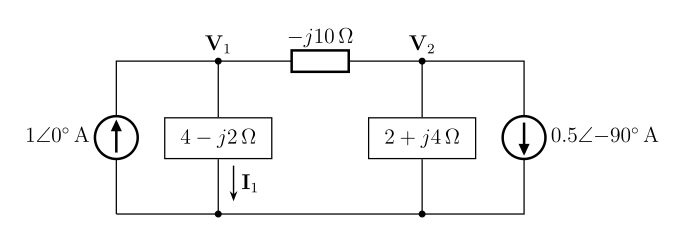
Circuit for the Thévenin equivalent.
Figure 9: Circuit for the Thévenin equivalent.

Let’s first disconnect the load:
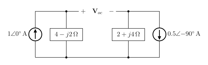
The circuit with the load disconnected.
Figure 10: The circuit with the load disconnected.

Which means VocV_{oc},

Voc=V1−V2=(1∠0∘)(4−j2)−(−0.5∠−90∘)(2−j4)=6−j3.\begin{align*} V_{oc} & = V_1 - V_2 \newline & = (1 \angle 0^{\circ})(4 - j2) - (-0.5 \angle -90^{\circ})(2 - j4) \newline & = 6 - j3. \end{align*}

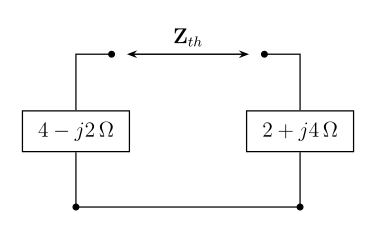
For our equivalent impedance:

The circuit with the sources turned off.
Figure 11: The circuit with the sources turned off.

Which means,

Zth=(4−j2)+(2+j4)=6+j2 Ω.\begin{align*} Z_{th} & = (4 - j2) + (2 + j4) \newline & = 6 + j2 \ \Omega. \end{align*}

Resonance

Definition 1 (Resonance)

A network is in resonance (or resonant) when the voltage and current at the network input terminals are in phase.

A maximum-amplitude response is produced in the resonant condition.
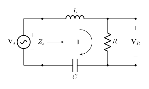
Series resonant circuit.
Figure 12: Series resonant circuit.

From this we can see that,

Zs=j2πfL+R−j12πfC.Z_{s} = j2\pi f L + R - j \dfrac{1}{2\pi f C}.

At the resonant frequency,

j2πf0L=j12πf0C,f0=12πLC.\begin{align*} j2\pi f_0 L & = j \dfrac{1}{2\pi f_0 C}, \newline f_0 & = \dfrac{1}{2\pi \sqrt{LC}}. \end{align*}

We call the ratio of the reactance of the impedance to the resistance at the resonant frequency the quality factor,

Qs=2πf0LR=12πf0CR.Q_{s} = \dfrac{2\pi f_0 L}{R} = \dfrac{1}{2\pi f_0 CR}.

Which means,

Zs=R[1+jQs(ff0−f0f)].Z_{s} = R\left[1 + jQ_s \left(\dfrac{f}{f_0} - \dfrac{f_0}{f}\right)\right]. I=VsZs=VsR[1+jQs(ff0−f0f)]I = \dfrac{V_s}{Z_s} = \dfrac{V_s}{R\left[1 + jQ_s \left(\dfrac{f}{f_0} - \dfrac{f_0}{f}\right)\right]} RI=Vs1+jQs(ff0−f0f)RI = \dfrac{V_s}{1 + jQ_s \left(\dfrac{f}{f_0} - \dfrac{f_0}{f}\right)} VRVs=11+jQs(ff0−f0f)\dfrac{V_R}{V_s} = \dfrac{1}{1 + jQ_s \left(\dfrac{f}{f_0} - \dfrac{f_0}{f}\right)} B=fH−fL=f0Qs.B = f_H - f_L = \dfrac{f_0}{Q_s}.

Search

Essays, lecture notes, and research

Type to search the site.