Part 8 - Magnetic fields | rezarezvan.com

In this part we’ll cover more in-depth about magnetic fields and their interactions.

Recall Biot-Savart’s Law,

\mathbf{\vec{B}} = \int d\mathbf{\vec{B}} = \dfrac{\mu_0 I}{4\pi} \int \dfrac{d\mathbf{\vec{s}} \times \hat{\mathbf{r}}}{r^2}.

This means that the magnetic field strength, $B$ , at any given point is,

B = \dfrac{\mu_0 I}{2\pi r}.

The direction, $\mathbf{\vec{B}}$ , is given by the (lazy) right-hand rule.

Magnetic field from a solenoid

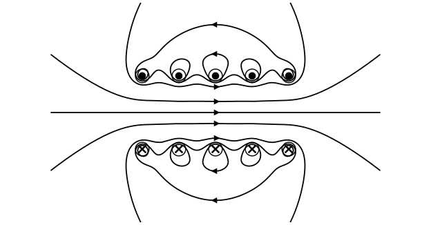
First, let’s draw how the field lines would look like:

Figure 1: Field lines of a solenoid, in cross-section.

If we zoom in, and look at the magnetic field on a square:

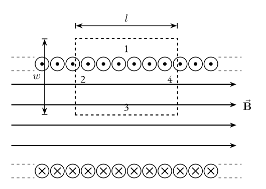
Figure 2: An Amperian loop over the solenoid.

If we write this as an integral,

\oint \mathbf{\vec{B}} \cdot d\mathbf{\vec{s}} = \int_1 \mathbf{\vec{B}} \cdot d\mathbf{\vec{s}} + \int_2 \mathbf{\vec{B}} \cdot d\mathbf{\vec{s}} + \int_3 \mathbf{\vec{B}} \cdot d\mathbf{\vec{s}} + \int_4 \mathbf{\vec{B}} \cdot d\mathbf{\vec{s}}.

But we can see that only $3$ will contribute to our magnetic field, since it’s parallel with it.

Which means,

\oint \mathbf{\vec{B}} \cdot d\mathbf{\vec{s}} = Bl = \mu_0 I_{enc}.

One thing we’ll need to remember is that, we can make our solenoid more densely coiled. This will, naturally, increase our magnetic field strength.

\begin{align*} I_{enc} & = NI, \newline \oint \mathbf{\vec{B}} \cdot d\mathbf{\vec{s}} & = Bl = \mu_0 NI. \end{align*}

Which means,

B = \dfrac{\mu_0 NI}{l} = \mu_0 nI,

where $n$ is the number of turns per length unit.

Lorentz Force

If we have a charged particle, in presence of both an electrical field, $\mathbf{\vec{E}}$ , and a magnetic field, $\mathbf{\vec{B}}$ .

The total force on the charged particle is, naturally, the sum of the two forces,

\begin{align*} \mathbf{\vec{F}}_E & = q\mathbf{\vec{E}}, \newline \mathbf{\vec{F}}_B & = q\mathbf{\vec{v}} \times \mathbf{\vec{B}}. \end{align*}

Theorem 1 (Lorentz force)

\mathbf{\vec{F}} = q(\mathbf{\vec{E}} + \mathbf{\vec{v}} \times \mathbf{\vec{B}})

Magnetic materials

As we have seen earlier, introduction of materials in electrical fields - always reduced the electrical field strength, $E$ .

However, we’ll see that, introduction of materials in a magnetic field may decrease or increase the magnetic field strength, $B$ .

To understand this - let’s begin with looking at this:

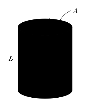
Here we have a cylinder with uniformly distributed magnetic dipoles.

The net dipole moment is,

\mathbf{\vec{M}} = \dfrac{1}{LA}\sum \vec{\boldsymbol{\mu}}_i.

Therefore, the magnetic field strength is just,

\mathbf{\vec{B}}_M = \mu_0 \mathbf{\vec{M}}.

However, these dipoles will probably not be uniformly distributed, rather quite chaotic and random. Thus, there is no net dipole moment.

If we however exert an external magnetic field, $\mathbf{\vec{B}}_0$ , these dipoles will begin to align and enhance the field.

\begin{align*} \mathbf{\vec{M}} & = \chi_m \dfrac{\mathbf{\vec{B}}_0}{\mu_0}, \newline \mathbf{\vec{B}} & = (1 + \chi_m) \mathbf{\vec{B}}_0 = \kappa_m \mathbf{\vec{B}}_0, \end{align*}

where $\kappa_m$ is the relative permeability of the material.

As we discussed earlier, materials that greatly enhance the magnetic field are called ferromagnetic materials.

The very cool and interesting thing is that, ferromagnetic materials induce the dipoles so strongly that, the dipoles themselves begin to strongly influence neighboring dipoles!

I find that very fascinating.

Faraday’s Law

From what we have assumed and used - our fields have been produced by stationary and moving charges.

Now, let’s do the opposite: varying a magnetic field with time to produce an electrical field.

To understand this we’ll first have to define magnetic flux.

Magnetic flux

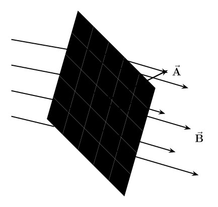
Just as electrical flux, we can define how much magnetic field passes through a surface.

Definition 1 (Magnetic flux)

We can define this as,

\Phi_B = \iint \mathbf{\vec{B}} \cdot d\mathbf{\vec{A}} = BA \cos(\theta).

The unit for magnetic flux is weber,

1 \ \mathrm{Wb} = 1 \ \mathrm{T \cdot m^2}.

Theorem 2 (Faraday’s law)

Now, back to Faraday’s law. The induced electromotive force, $\varepsilon$ , in a coil is proportional to the negative rate of change of the magnetic flux.

Or, in symbols,

\varepsilon = -N \dfrac{d \Phi_B}{dt},

where $N$ is the number of loops in the coil.

This also means that,

\varepsilon \propto - \dfrac{d}{dt} (BA \cos(\theta)).

We can also write this as,

-\left(\dfrac{dB}{dt}\right) A \cos(\theta) - \left(\dfrac{dA}{dt}\right) B \cos(\theta) + \left(\dfrac{d\theta}{dt}\right) BA \sin(\theta).

Here, we can clearly see that the induced electromotive force depends on the magnetic field, the area and the angle!

The direction of the induced current is determined by Lenz’s law, which says the following:

Theorem 3 (Lenz’s law)

The induced current produces a magnetic field, which opposes the change in magnetic flux that induces such currents.

Generators and motors

As the magnetic flux changes with time, an induced current begins to flow!

This, naturally, suggests that a potential difference is at play,

\begin{align*} \varepsilon & = \Delta V = \oint \mathbf{\vec{E}} \cdot d\mathbf{\vec{s}}, \newline \oint \mathbf{\vec{E}} \cdot d\mathbf{\vec{s}} & = - \dfrac{d \Phi_B}{dt}. \end{align*}

Now, by using Faraday’s law - we can design generators, to convert mechanical energy into electrical energy and vice versa!

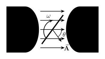
\Phi_B = \iint \mathbf{\vec{B}} \cdot d\mathbf{\vec{A}} = BA \cos(\theta) = BA \cos(\omega t)

Figure 5: A loop rotating in a magnetic field.

If we take the derivative,

\dfrac{d \Phi_B}{dt} = -BA \omega \sin(\omega t).

Therefore,

\varepsilon = -N \dfrac{d \Phi_B}{dt} = NBA \omega \sin(\omega t).

And also,

I = \dfrac{|\varepsilon|}{R} = \dfrac{NBA \omega}{R} \sin(\omega t).

Finally, we have defined, alternating current. We’ll start to dive into this world into the future parts.

One last interesting formula that we’re going to look at,

P = I |\varepsilon| = \dfrac{(NBA \omega)^2}{R} \sin^2 (\omega t).

We can see that, it’s just the absolute value of the alternating current!