Part 9 - Electromagnetic Waves

In this part we’ll cover electromagnetic waves - we’ll see why electrical and magnetic fields always appear together.

Displacement current

If we recall Faraday’s law,

\oint \mathbf{\vec{E}} \cdot d\mathbf{\vec{s}} = -\dfrac{d \Phi_B}{dt}.

This says that a change in the magnetic field will produce an electrical field. But how about the converse?

Does a change in an electrical field produce a magnetic field?

If we consider this example with a capacitor being charged:

Figure 1: Two surfaces bounded by the same curve around a charging capacitor.

Using Ampere’s law,

\oint \mathbf{\vec{B}} \cdot d\mathbf{\vec{s}} = \mu_0 I_{enc}.

If we look at $S_1$ , we see that $I_{enc} = I$ - however, for $S_2$ , $I_{enc} = 0$ - but the current does continue?

So we will need to add an extra term to Ampere’s law,

\oint \mathbf{\vec{B}} \cdot d\mathbf{\vec{s}} = \mu_0(I + I_d),

Definition 1 (Displacement current)

where the displacement current, $I_d$ , is

I_d = \varepsilon_0 \dfrac{d \Phi_E}{dt}.

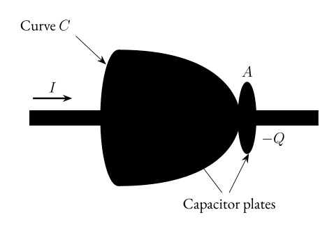
In practice, $I = I_d$ , thus the choice of the Amperian loop is inconsequential!

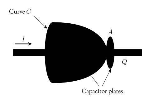
Figure 2: The changing electrical field between the plates.

Gauss’s Law

For electrostatics, Gauss’s law said that,

\Phi_E = \oiint \mathbf{\vec{E}} \cdot d\mathbf{\vec{A}} = \dfrac{q}{\varepsilon_0}.

But in the case for magnetism - magnetic monopoles do not exist (meaning that $q = 0$ ). Therefore,

\Phi_B = \oiint \mathbf{\vec{B}} \cdot d\mathbf{\vec{A}} = 0.

Maxwell’s Equations

With these new tools in mind - we have now learned the four Maxwell equations that form the basis of electromagnetism!

Let’s write them all down:

Theorem 1 (Maxwell’s equations)

Gauss’s Law for electrostatics:

\Phi_E = \oiint \mathbf{\vec{E}} \cdot d\mathbf{\vec{A}} = \dfrac{q}{\varepsilon_0}

Gauss’s Law for magnetism:

\Phi_B = \oiint \mathbf{\vec{B}} \cdot d\mathbf{\vec{A}} = 0

Faraday’s Law:

\varepsilon = \oint \mathbf{\vec{E}} \cdot d\mathbf{\vec{s}} = -\dfrac{d \Phi_B}{dt}

Ampere-Maxwell Law:

\oint \mathbf{\vec{B}} \cdot d\mathbf{\vec{s}} = \mu_0(I + I_d) = \mu_0\left(I + \varepsilon_0 \dfrac{d \Phi_E}{dt}\right)

If sources are absent (meaning that $q = 0$ and $I = 0$ ) - all of these become quite compact and tidy:

Gauss’s Law for electrostatics:

\Phi_E = \oiint \mathbf{\vec{E}} \cdot d\mathbf{\vec{A}} = 0

Gauss’s Law for magnetism:

\Phi_B = \oiint \mathbf{\vec{B}} \cdot d\mathbf{\vec{A}} = 0

Faraday’s Law:

\varepsilon = \oint \mathbf{\vec{E}} \cdot d\mathbf{\vec{s}} = -\dfrac{d \Phi_B}{dt}

Ampere-Maxwell Law:

\oint \mathbf{\vec{B}} \cdot d\mathbf{\vec{s}} = \mu_0 \varepsilon_0 \dfrac{d \Phi_E}{dt}

Now we can see, from Faraday’s law and Ampere-Maxwell’s Law that, if we have a change in one field - we’ll see a change in the other!

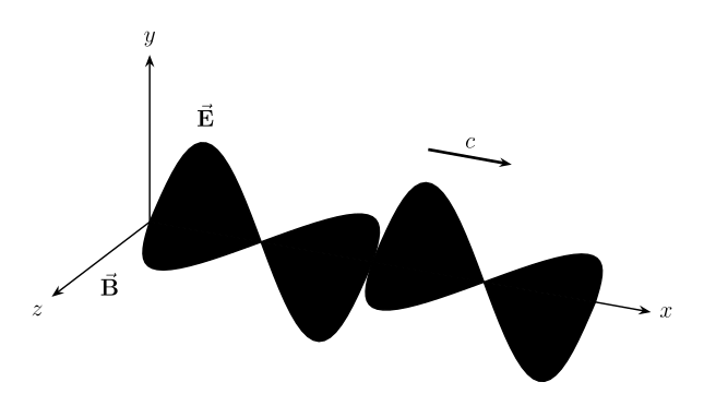
We’ll see why this picture will make a lot of sense soon:

Inductance

We have seen some aspects of inductance already - the induced current.

Imagine this scenario:

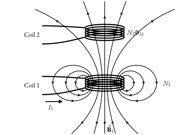
Figure 4: The field of coil 1 passes through coil 2.

We can see that our $\mathbf{\vec{B}}_1$ passes through the second coil, therefore a flux is generated, $\Phi_{21}$ .

As we learned last time, varying $I_1$ will induce an emf!

Which means,

\varepsilon_{21} = -N_2 \dfrac{d \Phi_{21}}{dt}.

If we want to write this in terms of $I_1$ we get,

\varepsilon_{21} = -M_{21} \dfrac{d I_1}{dt},

where $M_{21}$ is,

M_{21} = \dfrac{N_2 \Phi_{21}}{I_1}.

But let’s say that we vary $I_2$ , this will also lead to an EMF, but in the first coil,

\varepsilon_{12} = -N_1 \dfrac{d \Phi_{12}}{dt} = -M_{12} \dfrac{d I_2}{dt}.

Then, if we use the theorem of reciprocity - which states that:

Theorem 2 (Reciprocity)

The current at one point in a circuit due to a voltage at a second point is the same as the current at the second point due to the same voltage at the first.

Using this and combining Ampere’s law and the Biot-Savart law - we get,

M_{12} = M_{21} = M.

This means - sending varying current (AC) through coil 1 - will generate an AC current in coil 2 as well!

We can also connect this to voltage, potential drop,

\dfrac{V_2}{V_1} = \dfrac{N_2}{N_1}.

Self-Inductance

Say we only have one coil.

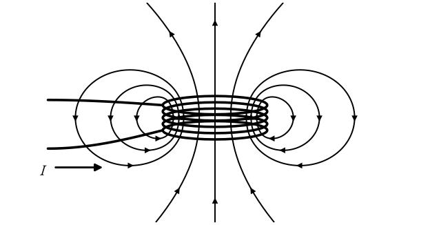
Figure 5: A single coil and its own field.

If we vary, $I$ , an induced EMF will oppose the change in flux, according to Faraday’s law.

We denote this self-induced EMF with $\varepsilon_L$ .

We can write it as,

\varepsilon_L = -N \dfrac{d \Phi_B}{dt}.

Definition 2 (Self-inductance)

We can relate this self-induced EMF with self-inductance, $L$ ,

\varepsilon_L = -L \dfrac{dI}{dt}.

We can also write,

L = \dfrac{N \Phi_B}{I} = \dfrac{\mu_0 N^2 A}{l}.

Therefore, the inductance, is a measure of an inductor’s resistance to change of the current!

In even simpler terms - inductors oppose change in the current!

So, since inductors oppose changes to the current - work must be done to establish a current in the inductor. Thus, energy must be stored in the magnetic field in an inductor! Similar to electrical fields in a capacitor.

The power, or the rate at which an external EMF, $\varepsilon_{ext}$ , works to overcome the self-induced EMF, $\varepsilon_L$ , to pass the current $I$ ,

P_L = \dfrac{d W_{ext}}{dt} = I \varepsilon_{ext} = -I \varepsilon_L = IL \dfrac{dI}{dt}.

This assumes that only $\varepsilon_{ext}$ and the inductor are present.

The total work done by an external source to increase the current from 0 to $I$ is,

W_{ext} = \int dW_{ext} = \int_0^I IL \, dI = \boxed{\dfrac{1}{2}LI^2}.

Electromagnetic waves

We’ll now cover a very cool phenomenon - we’ll cover why electromagnetic waves travel at light speed!

To prove this we’ll need to rewrite our definition for $\mathbf{\vec{E}}$ and $\mathbf{\vec{B}}$ ,

\begin{align*} \mathbf{\vec{E}} & = E_y(x, t) \hat{\mathbf{j}} = E \cos(kx - \omega t) \hat{\mathbf{j}}, \newline \mathbf{\vec{B}} & = B_z(x, t) \hat{\mathbf{k}} = B \cos(kx - \omega t) \hat{\mathbf{k}}. \end{align*}

Using Faraday’s law,

\oint \mathbf{\vec{E}} \cdot d\mathbf{\vec{s}} = - \dfrac{d}{dt} \iint \mathbf{\vec{B}} \cdot d\mathbf{\vec{A}}.

If we take our ring integral inside an arbitrary rectangle - on the $xy$ -plane:

A rectangular loop in the xy-plane. — Figure 6: A rectangular loop in the $xy$ -plane.

\left(E_y(x + \Delta x) - E_y(x)\right) \Delta y = - \dfrac{d}{dt} \iint B_z \, dx \, dy.

We get that,

\dfrac{\partial E_y}{\partial x} = - \dfrac{\partial B_z}{\partial t}.

Let’s calculate both,

\begin{align*} \dfrac{\partial E_y}{\partial x} & = -kE \sin(kx - \omega t), \newline \dfrac{\partial B_z}{\partial t} & = \omega B \sin(kx - \omega t). \end{align*}

Which, finally, means,

\boxed{\dfrac{E}{B} = \dfrac{\omega}{k} = c}.

EMFs in circuits

Now that we have learned this beauty of electromagnetic waves - let’s tie it back to our electrical circuits.

As we learned with electrical fields and capacitors:

Recall

Electrical field opposes change in voltage.

\begin{align*} C & = \varepsilon_0 \dfrac{A}{d}, \newline U & = \dfrac{1}{2} C V^2, \newline I(t) & = C \dfrac{dV}{dt}. \end{align*}

We have now seen that, magnetic fields and inductors:

Recall

Magnetic field opposes change in the current.

\begin{align*} L & = \mu_0 N^2 \dfrac{A}{l}, \newline U & = \dfrac{1}{2} LI^2, \newline V(t) & = L \dfrac{dI}{dt}. \end{align*}

We can now use this knowledge to understand LC and RLC circuits - and see how and why the energy oscillates between the electrical and magnetic field!